Visualizes cell-level statistics — counts, fractions, and composition — across cell identities and metadata groupings. This is the primary function for exploring the distribution of cell types, clusters, and categorical metadata in single-cell transcriptomics datasets. It answers questions such as: "What proportion of each cell type is in each condition?", "How do cluster abundances change across samples?", and "What is the clonal composition within each cell type?"
CellStatPlot serves as a unified interface across 15+ visualization
types, all driven by a common data aggregation and fraction-calculation
pipeline. It supports four single-cell data containers:
Seurat objects — Extracts
@meta.data; usesIdents()as the default identity whenident = NULL.Giotto objects — Extracts cell metadata via
getCellMetadata()usingspat_unitandfeat_type.h5ad files (.h5ad or opened
H5File) — Reads fromobsviah5group_to_dataframe().Data frames — Internal method; all other methods ultimately delegate here after metadata extraction.
Usage
CellStatPlot(
  object,
  ident = NULL,
  group_by = NULL,
  group_by_sep = "_",
  spat_unit = NULL,
  feat_type = NULL,
  split_by = NULL,
  split_by_sep = "_",
  facet_by = NULL,
  rows_by = NULL,
  columns_split_by = NULL,
  frac = c("none", "group", "ident", "cluster", "all"),
  name = NULL,
  agg = "n()",
  plot_type = c("bar", "circos", "pie", "pies", "ring", "donut", "trend", "area",
    "sankey", "alluvial", "heatmap", "radar", "spider", "violin", "box"),
  swap = FALSE,
  ylab = NULL,
  ...
)
Arguments
- object
A Seurat object, a Giotto object, a path to an
.h5adfile, an openedH5Filefrom the hdf5r package, or a data frame (internal method) containing cell metadata.- ident
The metadata column containing cell identities (clusters, cell types). If
NULLfor a Seurat object, the active identity is used and stored under the column name"Identity". Required for Giotto and h5ad objects. This column forms the primary categorical axis of the plot — typically the x-axis, pie slices, or heatmap rows.- group_by
The metadata column(s) used for secondary grouping (conditions, samples, stimulation status). Default is
NULL. Behavior varies by plot type:For most plots, multiple columns are concatenated into a single grouping variable (separated by
group_by_sep).For
"sankey"and"heatmap"plots, multiple columns are NOT concatenated — each column forms a separate node or column grouping.For
"violin"and"box"plots, at most 2 columns are allowed: the first determines the x-axis breakdown, the second is passed asgroup_byto the underlying plot function.
- group_by_sep
Separator used when concatenating multiple
group_bycolumns into a single variable. Default is"_". Ignored for"sankey"and"heatmap"plots where columns are not combined.- spat_unit
Spatial unit name for Giotto objects (e.g.,
"cell"). Ignored for non-Giotto inputs. IfNULL, auto-detected viaGiottoClass::set_default_spat_unit().- feat_type
Feature type name for Giotto objects (e.g.,
"rna","dna","protein"). Ignored for non-Giotto inputs. IfNULL, auto-detected viaGiottoClass::set_default_feat_type().- split_by
Metadata column(s) used to split the data into separate plots. Each unique value (or combination) produces an independent plot. Multiple columns are concatenated using
split_by_sep. Default isNULL(no splitting).- split_by_sep
Separator used when concatenating multiple
split_bycolumns. Default is"_".- facet_by
Metadata column(s) used to facet the plots (separate panels within the same output). Not available for
"circos","sankey", and"heatmap"plot types. Default isNULL.- rows_by
Metadata column(s) used as the rows for
"heatmap"or"pies"plots. For"pies", this defines what each pie chart represents (e.g., clones). For"heatmap", this overrides the default row grouping (which would otherwise beident). When multiple columns are provided, they must be logical or numeric. Default isNULL.- columns_split_by
Metadata column used to split the columns of
"heatmap"or"pies"plots. This adds an additional level of column faceting beyond whatgroup_byprovides. Default isNULL.- frac
The fraction normalization mode. One of
"none"(default),"group","ident","cluster"(alias for"ident"), or"all". Fractions are calculated within eachsplit_byandfacet_bysubset. See the Fraction calculation section for detailed semantics.- name
Display name for the main legend / value scale in
"heatmap"and"pies"plots. Default isNULL, which auto-generates a name based on the fraction mode.- agg
An expression string passed to
dplyr::summarise()to compute the value for each ident-by-group intersection. Default is"n()"(count of cells). For example,"sum(hasTCR) / n()"computes the fraction of TCR-positive cells. Ignored for"circos"and"pies"plot types. See the Custom aggregation section for more examples.- plot_type
The visualization type. One of:
"bar"(default),"circos","pie","pies","ring"/"donut","trend","area","sankey"/"alluvial","heatmap","radar","spider","violin", or"box". See the Plot types section for guidance on choosing a type. Note:"donut"is an alias for"ring";"alluvial"is an alias for"sankey".- swap
Whether to exchange the roles of
identandgroup_by. Default isFALSE. Behavior by plot type:"bar","trend","area","ring","radar","spider": Putsgroup_byon the x-axis and usesidentfor fill/color."circos": Reverses the direction of edges (from ident to group_by instead of group_by to ident)."pies": Swapsgroup_byandidentfor the column grouping and pie grouping respectively."heatmap": Swapsgroup_byandcolumns_split_by(requirescolumns_split_byto be set)."violin","box": Swaps the x-axis andgroup_byassignments from the twogroup_bycolumns.
Only works when
group_byis specified. Note thatswapis different fromflip(which transposes coordinates).- ylab
Y-axis label. Default is
NULL, which auto-generates a label based on the fraction mode (e.g.,"Number of cells"or"Fraction of cells").- ...
Additional arguments passed to the underlying plotthis plotting function. The target function depends on
plot_type:"bar"—plotthis::BarPlot()(position,palette,alpha,x_text_angle, ...)"circos"—plotthis::CircosPlot()(labels_rot,links_alpha, ...)"pie"—plotthis::PieChart()"ring"/"donut"—plotthis::RingPlot()(palette,alpha, ...)"trend"—plotthis::TrendPlot()(palette,point_size,line_width, ...)"area"—plotthis::AreaPlot()(palette,alpha, ...)"sankey"/"alluvial"—plotthis::SankeyPlot()(links_alpha,links_fill_by, ...)"heatmap"—plotthis::Heatmap()(palette,cluster_rows,cluster_columns,show_row_names,show_column_names,cell_type, ...)"pies"—plotthis::Heatmap()(withcell_type = "pie";pie_size,pie_values,row_names_side,column_names_side, ...)"radar"—plotthis::RadarPlot()"spider"—plotthis::SpiderPlot()"violin"—plotthis::ViolinPlot()(add_box,comparisons,aspect.ratio, ...)"box"—plotthis::BoxPlot()(comparisons,aspect.ratio, ...)
Common layout parameters (
split_by,facet_by,combine,nrow,ncol) are handled byCellStatPlotdirectly.
Details
See:
for examples of using this function with a Giotto object.
And see:
for examples of using this function with .h5ad files.
Note
Default y-axis label: When ylab = NULL, the label is
auto-generated as "Number of cells" (when frac = "none") or
"Fraction of cells" (otherwise). Override with ylab for custom
labels.
Heatmap/pies metadata columns: When multiple rows_by columns are
specified for "heatmap" or "pies" plots, each column must be logical
or numeric. The function filters cells where the column is TRUE or
greater than zero.
Facet restrictions: facet_by is not supported for "circos",
"sankey", and "heatmap" plot types. For heatmaps, use
split_by to create separate plots.
Factor ordering: The order of categories in plots follows the factor levels of the metadata columns. Set factor levels before plotting to control the display order of cell types and groups.
Giotto spatial units and feature types: The spat_unit and
feat_type parameters are required to locate the correct metadata
within Giotto's hierarchical spatial data structure. When NULL,
Giotto's own default resolution is used.
Plot types
The plot_type parameter selects the visualization. Plot types fall into
several conceptual categories:
Composition within groups (requires group_by):
"bar"— Grouped or stacked bar chart. The default and most common choice. Shows count or fraction per ident, colored by group."trend"— Line chart connecting points across idents. Best for showing trends across ordered categories (e.g., pseudotime bins, dose levels)."area"— Stacked area chart. Similar to trend but emphasizes the cumulative composition."ring"/"donut"— Ring (donut) chart. A radial alternative to stacked bars.fracis forced to"group"."radar"— Radar chart showing each ident as an axis. Compact for comparing group profiles across multiple idents."spider"— Spider chart with filled polygons. Similar to radar but emphasizes the area covered by each group.
Flow between categories (requires group_by):
"circos"— Circos plot showing directed edges from one category to another (e.g., cluster to condition)."sankey"/"alluvial"— Sankey (alluvial) diagram for multi-step categorical flows. Supports multiplegroup_bycolumns to show cascading relationships.
Single-group composition (no group_by):
"pie"— Pie chart of cell counts per ident. Use for a quick overview of cluster proportions.
Matrix views (requires group_by):
"heatmap"— Heatmap of counts or fractions with idents as rows andgroup_bycategories as columns. Supports row splitting viarows_split_byand column splitting viacolumns_split_by."pies"— Heatmap where each cell is a pie chart showing sub-composition (e.g., clone distribution within each cluster-by-condition intersection). Requiresrows_by.
Distribution within idents (requires group_by):
"violin"— Violin plot showing the distribution of values per ident, grouped or split by metadata."box"— Box plot with the same structure as violin.
Fraction calculation
The frac parameter controls how cell counts are normalized:
"none"— Raw cell counts (default). The y-axis shows the absolute number of cells."group"— Fraction within each group. The total across all idents within each group sums to 1. Answers: "Of the cells in condition X, what fraction are each cell type?""ident"— Fraction within each ident. The total across all groups within each ident sums to 1. Answers: "Of the Beta cells, what fraction are in each condition?" Requiresgroup_by."cluster"— Alias for"ident"."all"— Fraction of all cells in the data (or split/facet subset). Answers: "What fraction of all cells are Beta cells in condition X?"
Fractions are calculated independently within each split_by and/or
facet_by subset.
Custom aggregation
By default, CellStatPlot counts the number of cells in each
ident-by-group intersection (agg = "n()"). The agg parameter accepts
any expression that can be passed to dplyr::summarise(), enabling
custom metrics. Examples:
"sum(hasTCR) / n()"— Fraction of cells with a TCR in each group"mean(expression_score)"— Mean of a numeric metadata column"sum(clone_size > 1)"— Number of expanded clones
Note: agg is ignored for "circos" and "pies" plot types, which
always count cells.
The ident/group_by duality
CellStatPlot is built around two categorical axes:
ident— The primary cell identity (clusters, cell types). This typically forms the x-axis, pie slices, or heatmap rows.group_by— A secondary grouping (conditions, samples, time points). This typically forms the fill colors, bar stacks, or heatmap columns.
The swap parameter exchanges these two roles: when swap = TRUE, the
group_by variable is used as the x-axis and ident provides the fill
colors. The exact behavior varies by plot type — see the swap
parameter documentation for details.
See also
CellDimPlot— Dimension reduction visualization of cell clustersFeatureStatPlot— Feature expression statisticsplotthis::BarPlot(),plotthis::Heatmap(),plotthis::SankeyPlot()— Underlying plotthis functions for individual plot types
Examples
# \donttest{
# library(patchwork)
data(ifnb_sub)
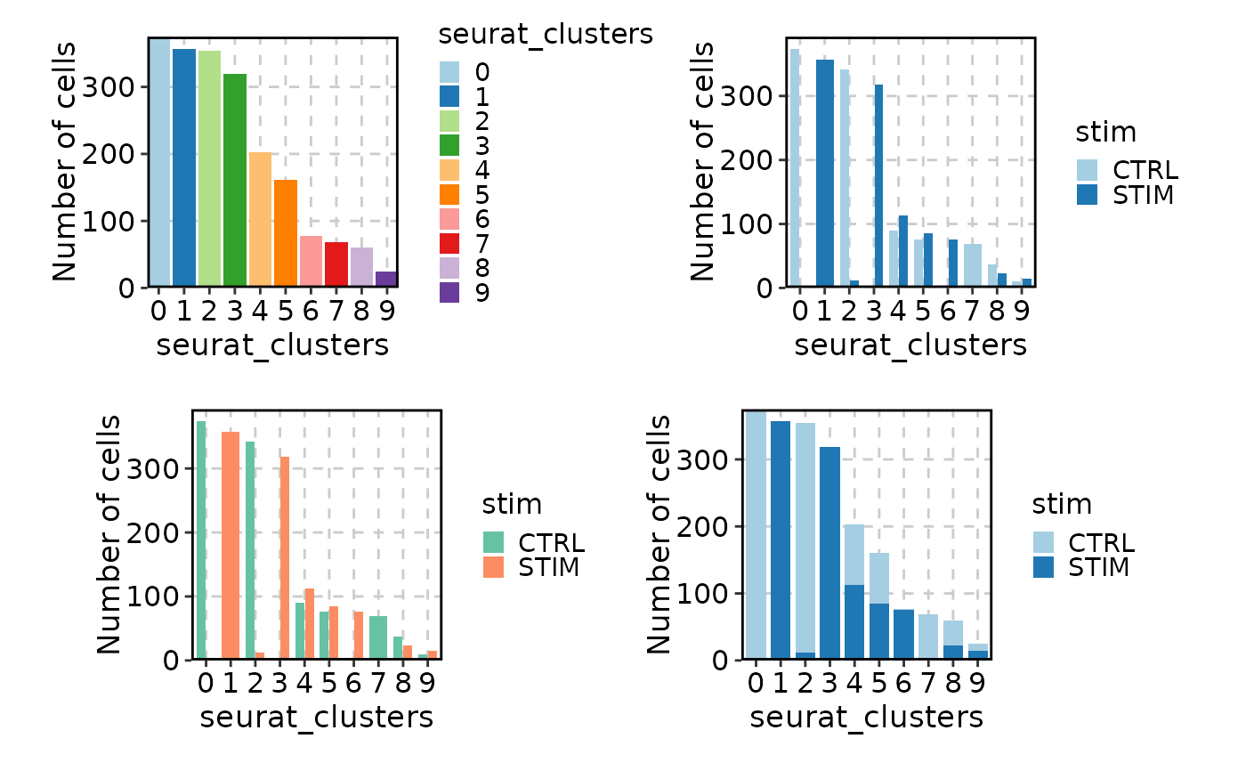
# Bar plot
p1 <- CellStatPlot(ifnb_sub)
p2 <- CellStatPlot(ifnb_sub, group_by = "stim")
p3 <- CellStatPlot(ifnb_sub, group_by = "stim", palette = "Set2")
p4 <- CellStatPlot(ifnb_sub, group_by = "stim", position = "stack")
(p1 | p2) / (p3 | p4)
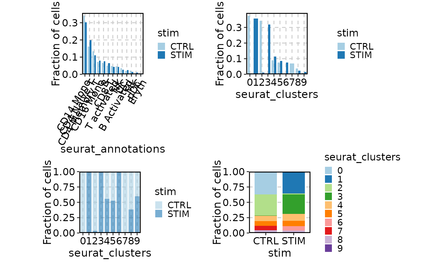
 # Fraction of cells
p1 <- CellStatPlot(ifnb_sub, group_by = "stim", frac = "group",
ident = "seurat_annotations", x_text_angle = 60)
p2 <- CellStatPlot(ifnb_sub, group_by = "stim", frac = "group")
p3 <- CellStatPlot(ifnb_sub, group_by = "stim", frac = "ident",
position = "stack", alpha = .6)
p4 <- CellStatPlot(ifnb_sub, group_by = "stim", frac = "group",
swap = TRUE, position = "stack")
(p1 | p2) / (p3 | p4)
# Fraction of cells
p1 <- CellStatPlot(ifnb_sub, group_by = "stim", frac = "group",
ident = "seurat_annotations", x_text_angle = 60)
p2 <- CellStatPlot(ifnb_sub, group_by = "stim", frac = "group")
p3 <- CellStatPlot(ifnb_sub, group_by = "stim", frac = "ident",
position = "stack", alpha = .6)
p4 <- CellStatPlot(ifnb_sub, group_by = "stim", frac = "group",
swap = TRUE, position = "stack")
(p1 | p2) / (p3 | p4)
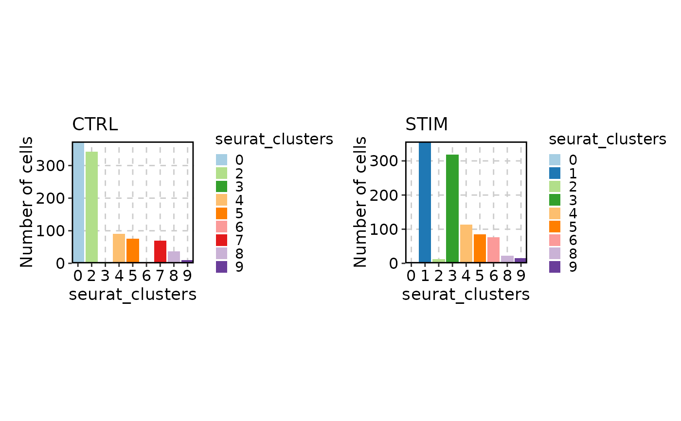
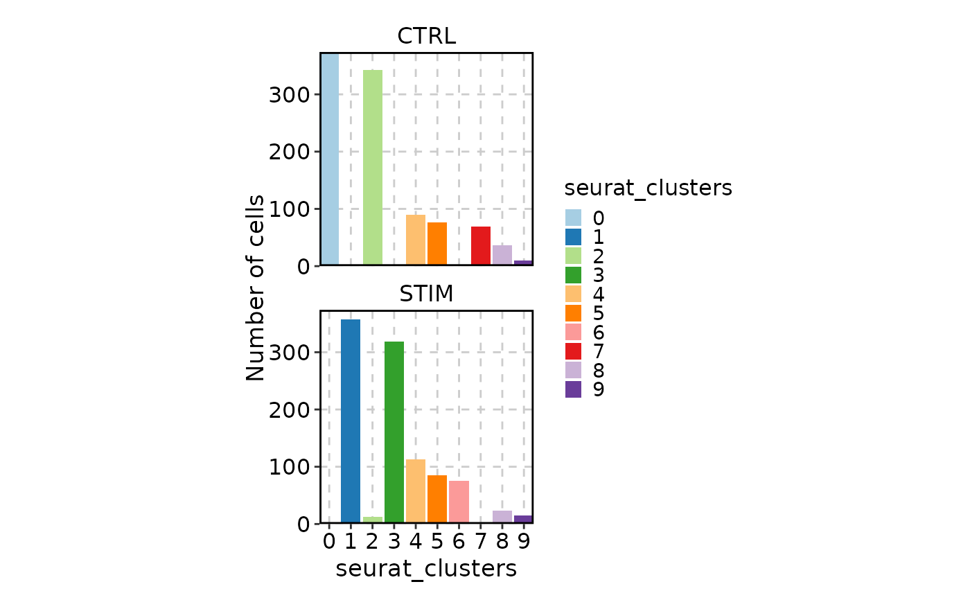
 # Splitting/Facetting the plot
CellStatPlot(ifnb_sub, split_by = "stim")
# Splitting/Facetting the plot
CellStatPlot(ifnb_sub, split_by = "stim")
 CellStatPlot(ifnb_sub, facet_by = "stim")
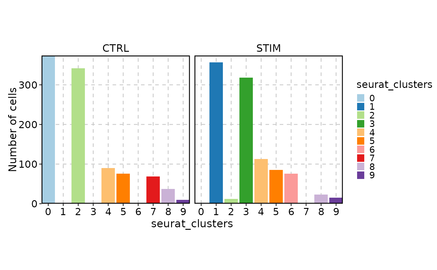 CellStatPlot(ifnb_sub, facet_by = "stim", facet_nrow = 2)
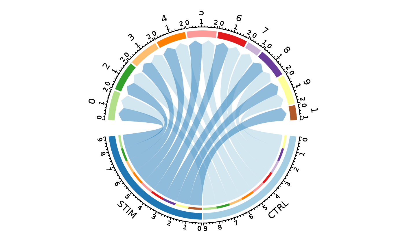
 # Circos plot
CellStatPlot(ifnb_sub, group_by = "stim", plot_type = "circos")
# Circos plot
CellStatPlot(ifnb_sub, group_by = "stim", plot_type = "circos")
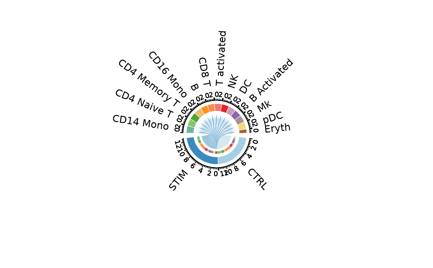
 CellStatPlot(ifnb_sub, group_by = "stim", ident = "seurat_annotations",
plot_type = "circos", labels_rot = TRUE)
CellStatPlot(ifnb_sub, group_by = "stim", ident = "seurat_annotations",
plot_type = "circos", labels_rot = TRUE)
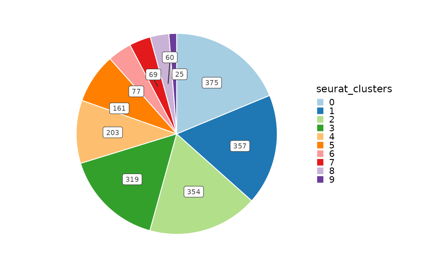
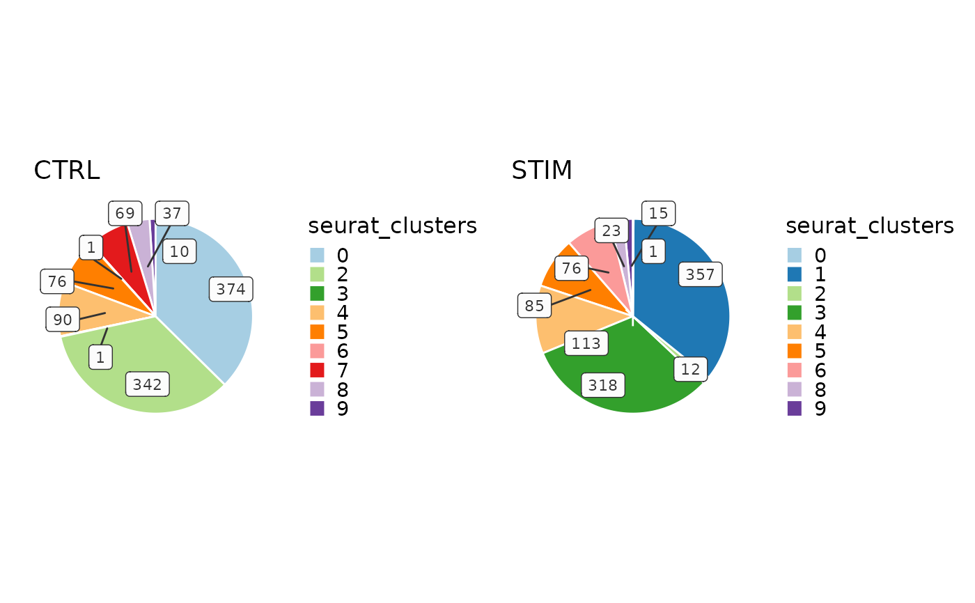
 # Pie plot
CellStatPlot(ifnb_sub, plot_type = "pie")
# Pie plot
CellStatPlot(ifnb_sub, plot_type = "pie")
 CellStatPlot(ifnb_sub, plot_type = "pie", split_by = "stim")
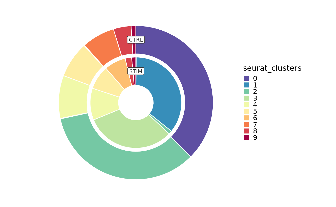
 # Ring plot
CellStatPlot(ifnb_sub, plot_type = "ring", group_by = "stim",
palette = "Spectral")
#> 'frac' is forced to 'group' for 'ring' plot.
# Ring plot
CellStatPlot(ifnb_sub, plot_type = "ring", group_by = "stim",
palette = "Spectral")
#> 'frac' is forced to 'group' for 'ring' plot.
 # Trend plot
CellStatPlot(ifnb_sub, plot_type = "trend", frac = "group",
x_text_angle = 90, group_by = c("stim", "seurat_annotations"))
#> Multiple columns are provided in 'group_by'. They will be concatenated into one column.
# Trend plot
CellStatPlot(ifnb_sub, plot_type = "trend", frac = "group",
x_text_angle = 90, group_by = c("stim", "seurat_annotations"))
#> Multiple columns are provided in 'group_by'. They will be concatenated into one column.
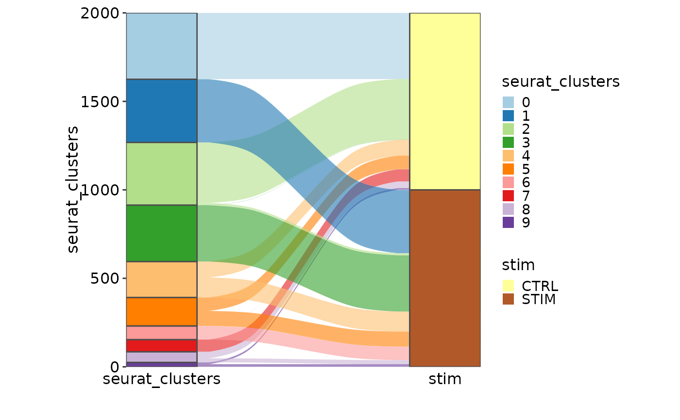
 # Sankey plot
CellStatPlot(ifnb_sub, plot_type = "sankey", group_by = c("seurat_clusters", "stim"),
links_alpha = .6)
#> Missing alluvia for some stratum combinations.
# Sankey plot
CellStatPlot(ifnb_sub, plot_type = "sankey", group_by = c("seurat_clusters", "stim"),
links_alpha = .6)
#> Missing alluvia for some stratum combinations.
 CellStatPlot(ifnb_sub, plot_type = "sankey", links_alpha = .6,
group_by = c("stim", "seurat_annotations", "orig.ident"))
#> Missing alluvia for some stratum combinations.
CellStatPlot(ifnb_sub, plot_type = "sankey", links_alpha = .6,
group_by = c("stim", "seurat_annotations", "orig.ident"))
#> Missing alluvia for some stratum combinations.
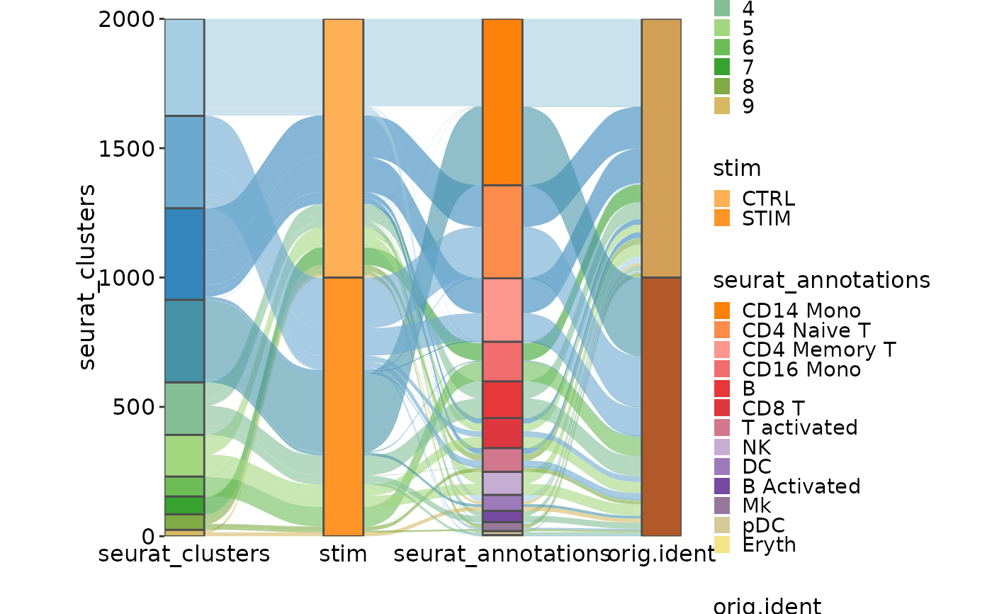 CellStatPlot(ifnb_sub, plot_type = "sankey", links_alpha = .6,
group_by = c("seurat_clusters", "stim", "seurat_annotations", "orig.ident"))
#> Missing alluvia for some stratum combinations.
CellStatPlot(ifnb_sub, plot_type = "sankey", links_alpha = .6,
group_by = c("seurat_clusters", "stim", "seurat_annotations", "orig.ident"))
#> Missing alluvia for some stratum combinations.
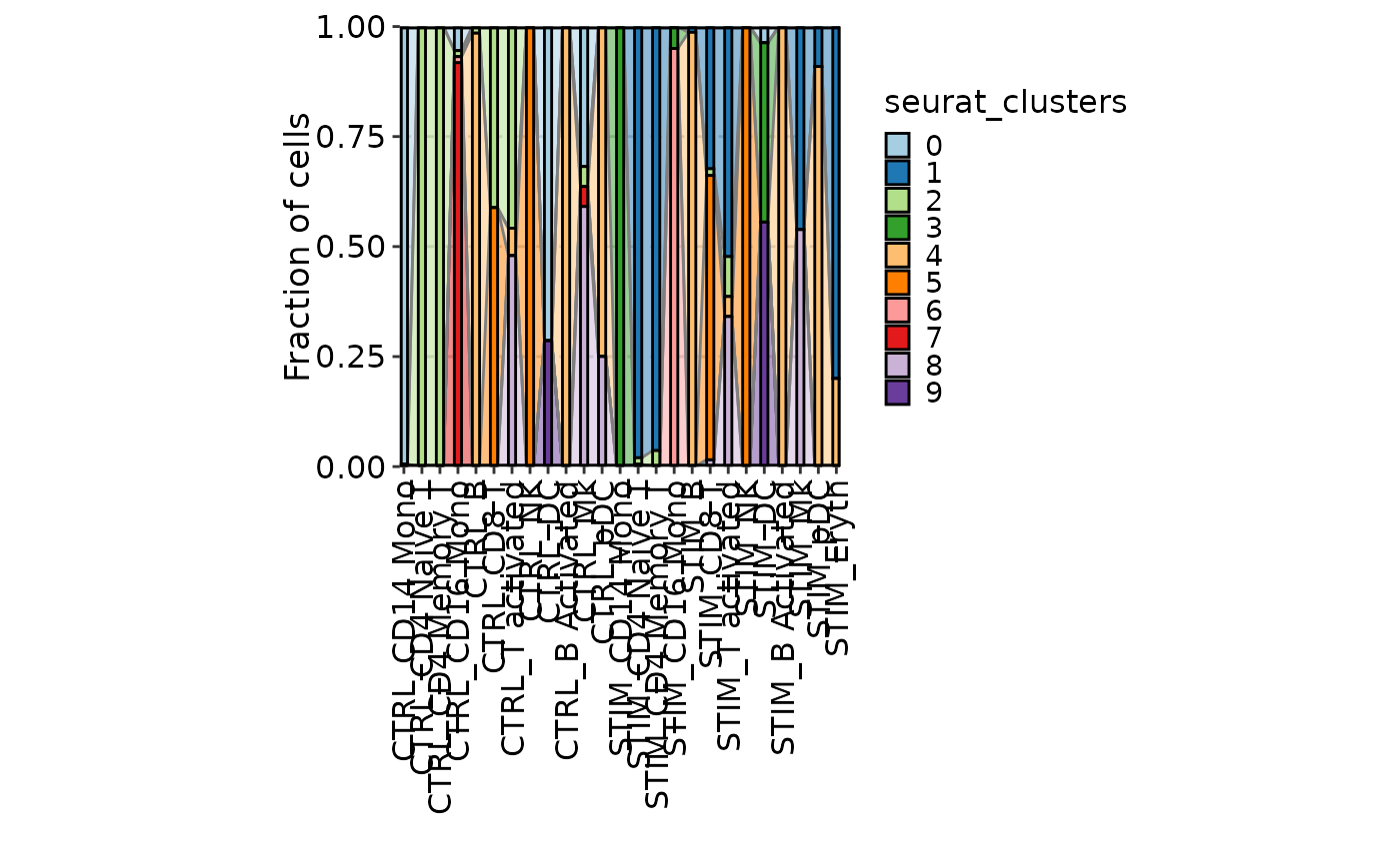
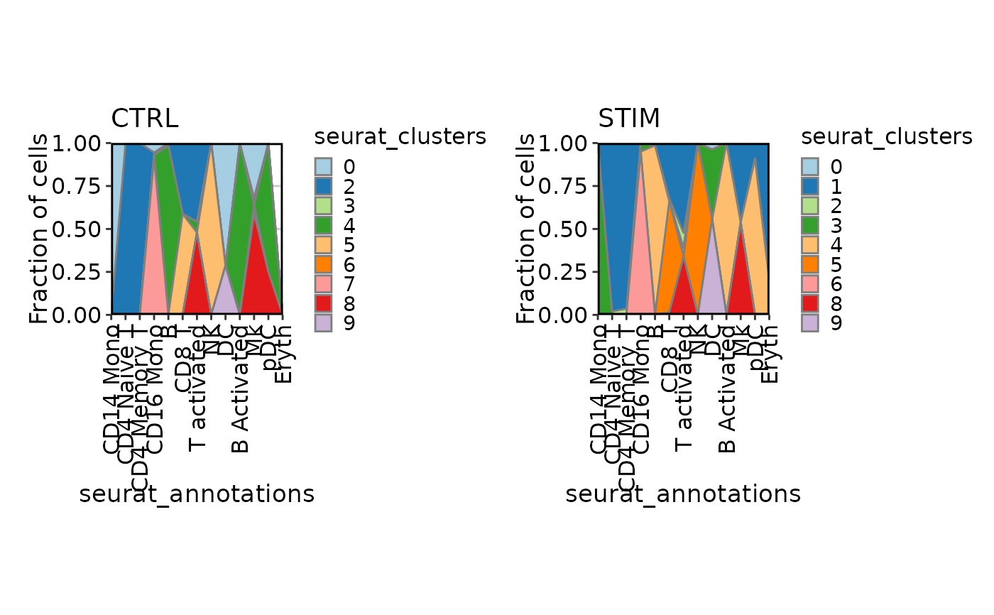 # Area plot
CellStatPlot(ifnb_sub, plot_type = "area", frac = "group", x_text_angle = 90,
group_by = "seurat_annotations", split_by = "stim")
# Area plot
CellStatPlot(ifnb_sub, plot_type = "area", frac = "group", x_text_angle = 90,
group_by = "seurat_annotations", split_by = "stim")
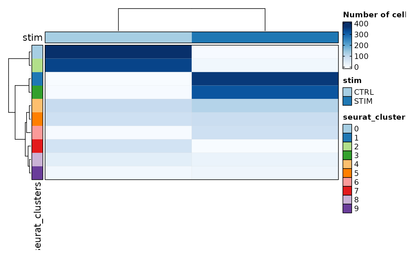
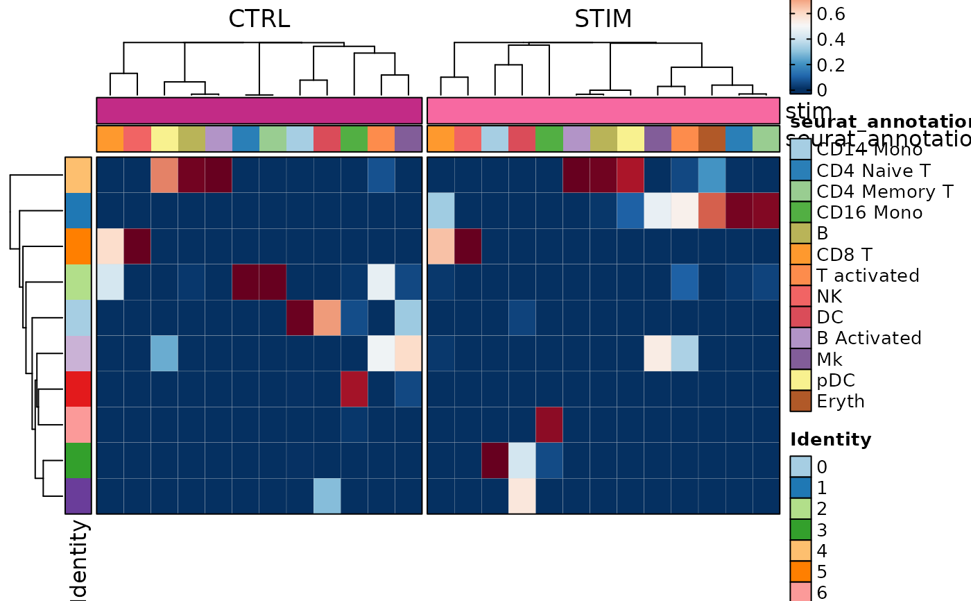
 # Heatmap
CellStatPlot(ifnb_sub, plot_type = "heatmap", group_by = "stim", palette = "Blues")
# Heatmap
CellStatPlot(ifnb_sub, plot_type = "heatmap", group_by = "stim", palette = "Blues")
 CellStatPlot(ifnb_sub, plot_type = "heatmap", group_by = "stim",
frac = "group", columns_split_by = "seurat_annotations", swap = TRUE)
CellStatPlot(ifnb_sub, plot_type = "heatmap", group_by = "stim",
frac = "group", columns_split_by = "seurat_annotations", swap = TRUE)
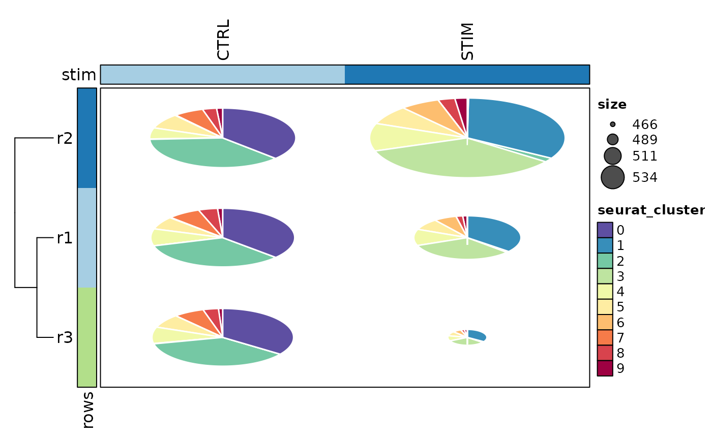
 # Pies
# Simulate some sets of cells (e.g. clones)
ifnb_sub$r1 <- ifelse(ifnb_sub$seurat_clusters %in% c("0", "1", "2"), 1, 0)
ifnb_sub$r2 <- sample(c(1, 0), ncol(ifnb_sub), prob = c(0.5, 0.5), replace = TRUE)
ifnb_sub$r3 <- sample(c(1, 0), ncol(ifnb_sub), prob = c(0.7, 0.3), replace = TRUE)
CellStatPlot(ifnb_sub, plot_type = "pies", group_by = "stim", rows_name = "Clones",
rows_by = c("r1", "r2", "r3"), column_names_side = "top", cluster_columns = FALSE,
row_names_side = "right", pie_size = "identity", pie_values = "sum")
# Pies
# Simulate some sets of cells (e.g. clones)
ifnb_sub$r1 <- ifelse(ifnb_sub$seurat_clusters %in% c("0", "1", "2"), 1, 0)
ifnb_sub$r2 <- sample(c(1, 0), ncol(ifnb_sub), prob = c(0.5, 0.5), replace = TRUE)
ifnb_sub$r3 <- sample(c(1, 0), ncol(ifnb_sub), prob = c(0.7, 0.3), replace = TRUE)
CellStatPlot(ifnb_sub, plot_type = "pies", group_by = "stim", rows_name = "Clones",
rows_by = c("r1", "r2", "r3"), column_names_side = "top", cluster_columns = FALSE,
row_names_side = "right", pie_size = "identity", pie_values = "sum")
 # Expand pies into heatmap
CellStatPlot(ifnb_sub, plot_type = "heatmap", group_by = "stim", rows_name = "Clones",
rows_by = c("r1", "r2", "r3"), column_names_side = "top", cluster_columns = FALSE,
row_names_side = "right")
# Expand pies into heatmap
CellStatPlot(ifnb_sub, plot_type = "heatmap", group_by = "stim", rows_name = "Clones",
rows_by = c("r1", "r2", "r3"), column_names_side = "top", cluster_columns = FALSE,
row_names_side = "right")
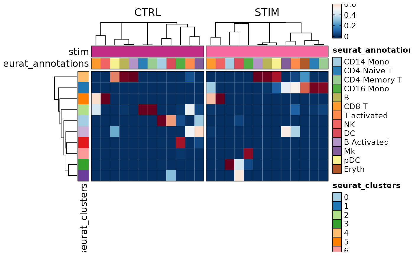
 # Rows split by clones instead of idents and show fraction of cells in each clone.
CellStatPlot(ifnb_sub, plot_type = "heatmap", group_by = "stim", frac = "group",
rows_split_by = c("r1", "r2", "r3"), column_names_side = "top", cluster_columns = FALSE,
row_names_side = "right", label = function(x) scales::number(x, accuracy = 0.01),
cell_type = "label")
# Rows split by clones instead of idents and show fraction of cells in each clone.
CellStatPlot(ifnb_sub, plot_type = "heatmap", group_by = "stim", frac = "group",
rows_split_by = c("r1", "r2", "r3"), column_names_side = "top", cluster_columns = FALSE,
row_names_side = "right", label = function(x) scales::number(x, accuracy = 0.01),
cell_type = "label")
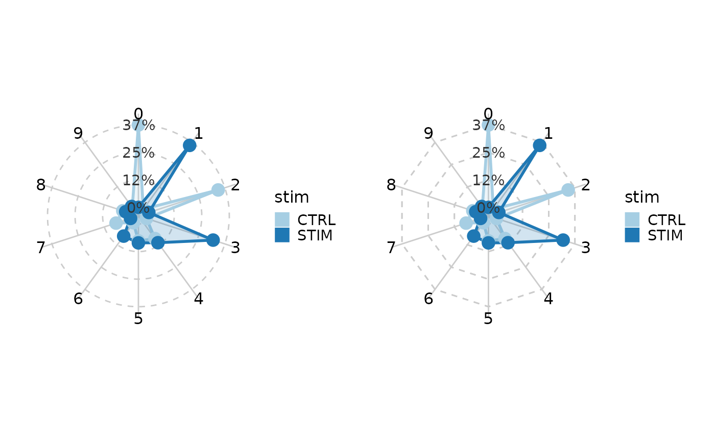
 # Radar plot/Spider plot
pr <- CellStatPlot(ifnb_sub, plot_type = "radar", group_by = "stim")
ps <- CellStatPlot(ifnb_sub, plot_type = "spider", group_by = "stim")
pr | ps
# Radar plot/Spider plot
pr <- CellStatPlot(ifnb_sub, plot_type = "radar", group_by = "stim")
ps <- CellStatPlot(ifnb_sub, plot_type = "spider", group_by = "stim")
pr | ps
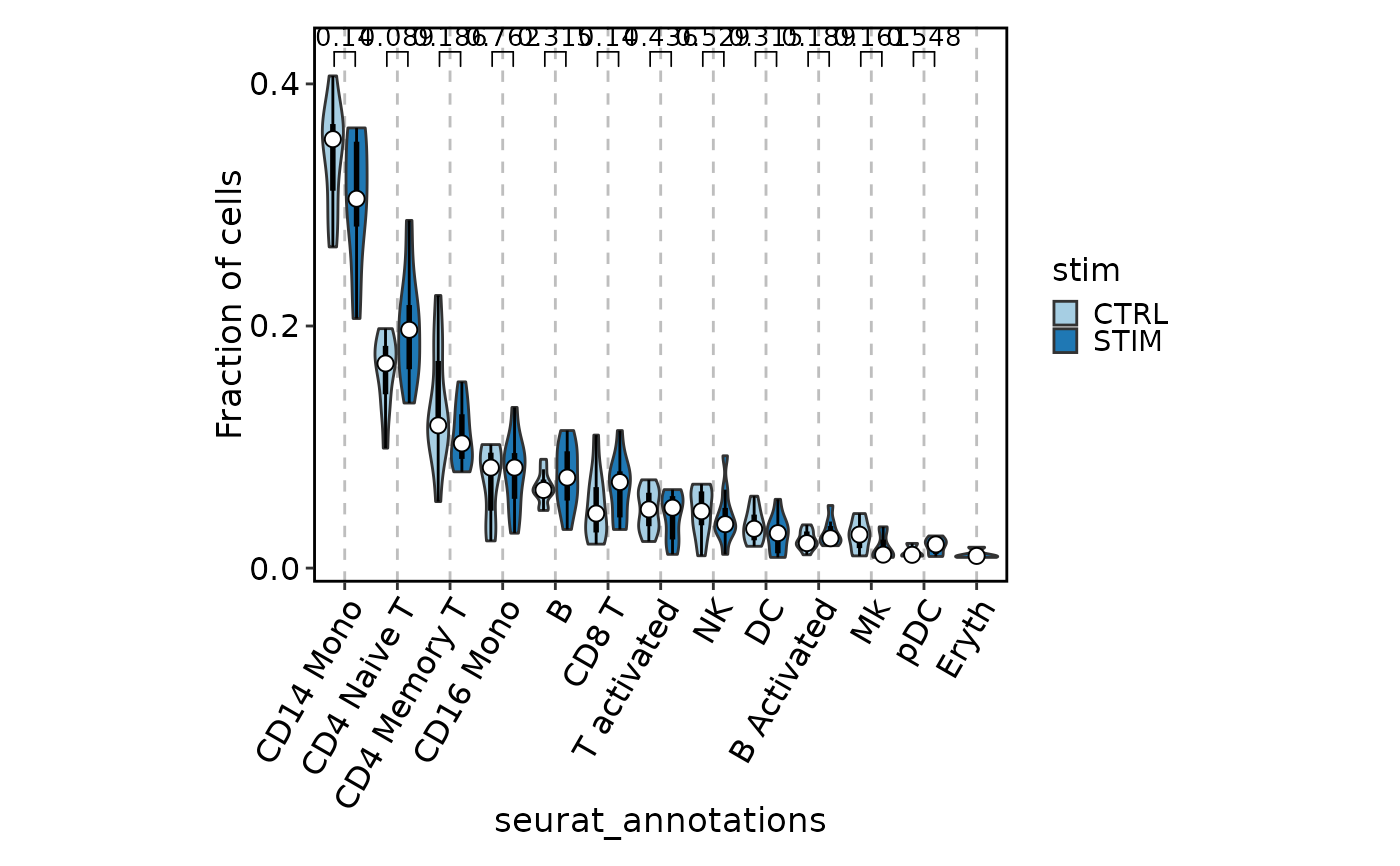
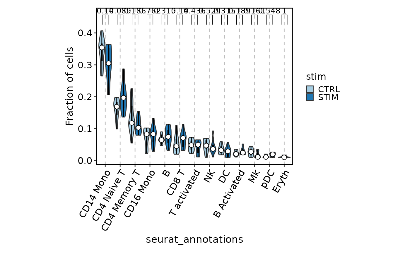
 # Box/Violin plot
ifnb_sub$group <- sample(paste0("g", 1:10), nrow(ifnb_sub), replace = TRUE)
CellStatPlot(ifnb_sub, group_by = c("group", "stim"), frac = "group",
plot_type = "violin", add_box = TRUE, ident = "seurat_annotations",
x_text_angle = 60, comparisons = TRUE, aspect.ratio = 0.8)
#> Warning: [Box/Violin/BeeswarmPlot] Some pairwise comparisons may fail due to insufficient data points or variability. Adjusting data to ensure valid comparisons.
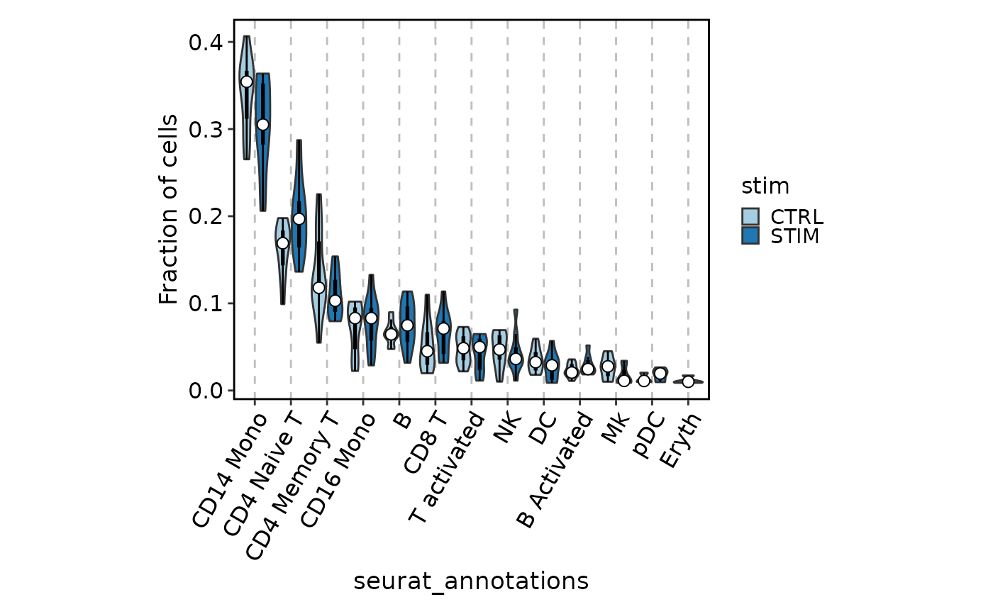
# Box/Violin plot
ifnb_sub$group <- sample(paste0("g", 1:10), nrow(ifnb_sub), replace = TRUE)
CellStatPlot(ifnb_sub, group_by = c("group", "stim"), frac = "group",
plot_type = "violin", add_box = TRUE, ident = "seurat_annotations",
x_text_angle = 60, comparisons = TRUE, aspect.ratio = 0.8)
#> Warning: [Box/Violin/BeeswarmPlot] Some pairwise comparisons may fail due to insufficient data points or variability. Adjusting data to ensure valid comparisons.
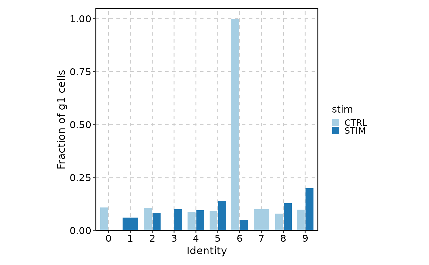
 # Use different agg other than counting the number of cells.
# Let's say we do the fraction of g1 in each stim group.
CellStatPlot(ifnb_sub, agg = "sum(group == 'g1') / n()",
plot_type = "bar", ylab = "Fraction of g1 cells")
# Use different agg other than counting the number of cells.
# Let's say we do the fraction of g1 in each stim group.
CellStatPlot(ifnb_sub, agg = "sum(group == 'g1') / n()",
plot_type = "bar", ylab = "Fraction of g1 cells")
 CellStatPlot(ifnb_sub, group_by = "stim", agg = "sum(group == 'g1') / n()",
plot_type = "bar", ylab = "Fraction of g1 cells")
CellStatPlot(ifnb_sub, group_by = "stim", agg = "sum(group == 'g1') / n()",
plot_type = "bar", ylab = "Fraction of g1 cells")
 # }
# }