
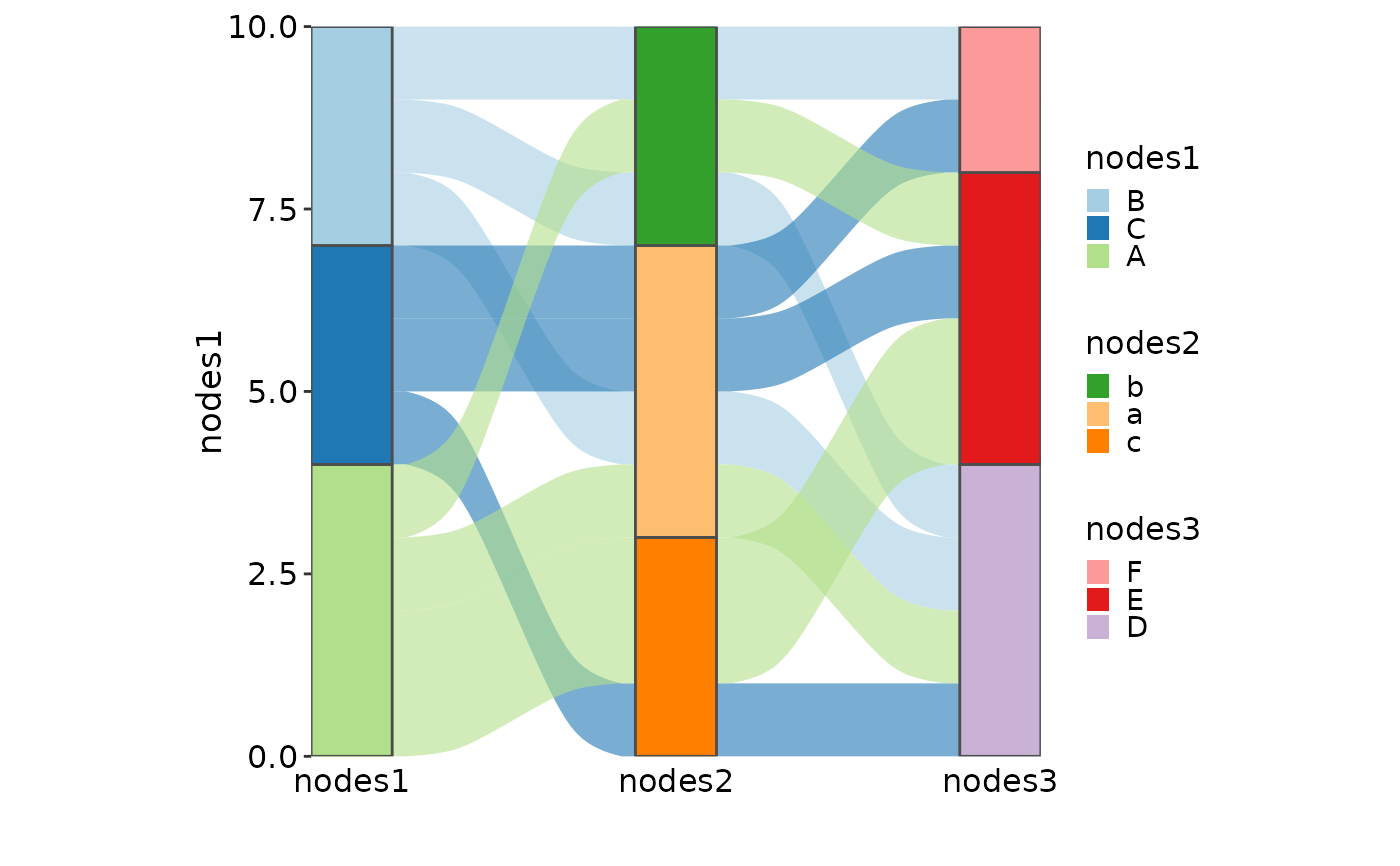
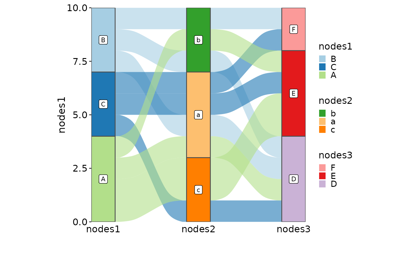
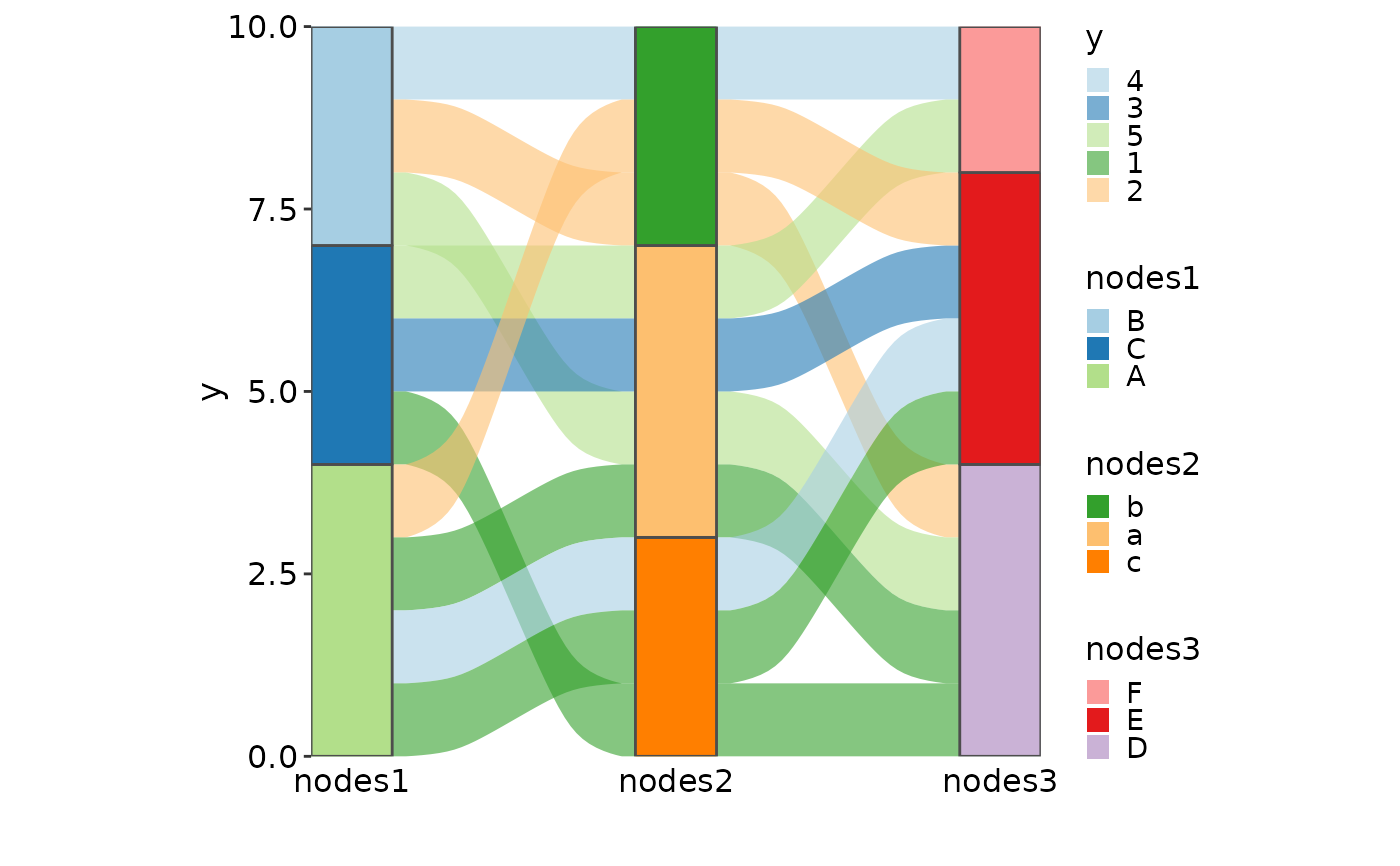
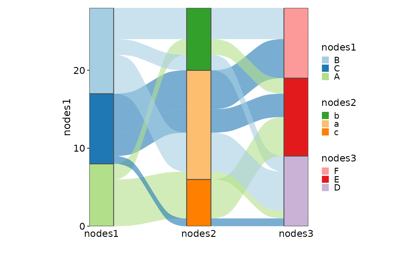
Draws Sankey (alluvial) diagrams to visualise flow, movement, or change from one categorical state to another across discrete positions (time points, stages, or groups). The plot consists of nodes (vertical blocks, or strata) representing categories at each position, and links (alluvia / flows) representing the observation units that move between categories across positions.
The function accepts data in several formats, controlled by in_form:
"lodes"/"long"Each row is an observation at one x-position, with columns for
x,stratum,alluvium, and optionallyy."alluvia"/"wide"Each row is an observation unit tracked across all positions;
xcolumns represent the categories at each position. Converted internally viato_lodes_form()."counts"Numeric columns under each
xrepresent frequencies. When the first element ofxis".", thelinks_fill_byvalues are injected as an additional first column of nodes, visualising the source distribution of flows."auto"(default)Automatically detects the format: numeric multi-column
x→"counts"; multi-columnxpassingis_alluvia_form→"alluvia"; otherwise →"lodes".
Supports split_by to produce separate sub-plots for different subsets of the data, facet_by for within-plot faceting, and independent styling of nodes and links (colours, alpha, borders, labels, and legend behaviour).
AlluvialPlot is an alias of SankeyPlot.
Usage
SankeyPlot(
  data,
  in_form = c("auto", "long", "lodes", "wide", "alluvia", "counts"),
  x,
  x_sep = "_",
  y = NULL,
  stratum = NULL,
  stratum_sep = "_",
  alluvium = NULL,
  alluvium_sep = "_",
  split_by = NULL,
  split_by_sep = "_",
  keep_empty = TRUE,
  flow = FALSE,
  expand = c(0, 0, 0, 0),
  nodes_legend = c("auto", "separate", "merge", "none"),
  nodes_color = "grey30",
  links_fill_by = NULL,
  links_fill_by_sep = "_",
  links_name = NULL,
  links_color = "gray80",
  nodes_palette = "Paired",
  nodes_palcolor = NULL,
  nodes_alpha = 1,
  nodes_label = FALSE,
  nodes_label_miny = 0,
  nodes_width = 0.25,
  links_palette = "Paired",
  links_palcolor = NULL,
  palreverse = FALSE,
  links_alpha = 0.6,
  legend.box = "vertical",
  x_text_angle = 0,
  aspect.ratio = 1,
  legend.position = "right",
  legend.direction = "vertical",
  flip = FALSE,
  theme = "theme_this",
  theme_args = list(),
  title = NULL,
  subtitle = NULL,
  xlab = NULL,
  ylab = NULL,
  facet_by = NULL,
  facet_scales = "fixed",
  facet_ncol = NULL,
  facet_nrow = NULL,
  facet_byrow = TRUE,
  seed = 8525,
  combine = TRUE,
  nrow = NULL,
  ncol = NULL,
  byrow = TRUE,
  axes = NULL,
  axis_titles = axes,
  guides = NULL,
  design = NULL,
  ...
)

AlluvialPlot(
  data,
  in_form = c("auto", "long", "lodes", "wide", "alluvia", "counts"),
  x,
  x_sep = "_",
  y = NULL,
  stratum = NULL,
  stratum_sep = "_",
  alluvium = NULL,
  alluvium_sep = "_",
  split_by = NULL,
  split_by_sep = "_",
  keep_empty = TRUE,
  flow = FALSE,
  expand = c(0, 0, 0, 0),
  nodes_legend = c("auto", "separate", "merge", "none"),
  nodes_color = "grey30",
  links_fill_by = NULL,
  links_fill_by_sep = "_",
  links_name = NULL,
  links_color = "gray80",
  nodes_palette = "Paired",
  nodes_palcolor = NULL,
  nodes_alpha = 1,
  nodes_label = FALSE,
  nodes_label_miny = 0,
  nodes_width = 0.25,
  links_palette = "Paired",
  links_palcolor = NULL,
  palreverse = FALSE,
  links_alpha = 0.6,
  legend.box = "vertical",
  x_text_angle = 0,
  aspect.ratio = 1,
  legend.position = "right",
  legend.direction = "vertical",
  flip = FALSE,
  theme = "theme_this",
  theme_args = list(),
  title = NULL,
  subtitle = NULL,
  xlab = NULL,
  ylab = NULL,
  facet_by = NULL,
  facet_scales = "fixed",
  facet_ncol = NULL,
  facet_nrow = NULL,
  facet_byrow = TRUE,
  seed = 8525,
  combine = TRUE,
  nrow = NULL,
  ncol = NULL,
  byrow = TRUE,
  axes = NULL,
  axis_titles = axes,
  guides = NULL,
  design = NULL,
  ...
)
Arguments
- data
A data frame.
- in_form
A character string specifying the input data format. One of
"auto"(default),"long","lodes","wide","alluvia", or"counts"."long"is an alias for"lodes";"wide"is an alias for"alluvia". See thedataparameter ofSankeyPlotfor format descriptions.- x
A character string specifying the column name of the data frame to plot for the x-axis.
- x_sep
A character string to join multiple
xcolumns whenin_formis"lodes"or auto-determined as lodes. Default"_".- y
A character string specifying the column name of the data frame to plot for the y-axis.
- stratum
A character string specifying the column that defines the node categories at each x-axis position. Each unique value becomes a stratum (node block) at each x position. When
NULL, defaults tolinks_fill_by. Multiple columns are concatenated withstratum_sep. Ignored in"alluvia"format.- stratum_sep
A character string to join multiple
stratumcolumns. Default"_".- alluvium
A character string specifying the column that identifies individual flows (alluvia) across x-axis positions. Each unique value represents a single observational unit tracked across positions. When
NULLin"counts"format, an auto-generated identifier is created. Multiple columns are concatenated withalluvium_sep. Ignored in"alluvia"format.- alluvium_sep
A character string to join multiple
alluviumcolumns. Default"_".- split_by
The column(s) to split data by and plot separately. When
combine = TRUE, the combined plot's data (p$data) contains the rows of every split, tagged with thesplit_bycolumn. For ggraph-based plots (e.g.Network,ClustreePlot), the node layout of every split is exposed with the split column, and the original link rows (also tagged with thesplit_bycolumn) are available as the"edges"attribute of the data.- split_by_sep
The separator for multiple split_by columns. See
split_by- keep_empty
One of FALSE, TRUE and "level". It can also take a named list to specify different behavior for different columns. Without a named list, the behavior applies to the categorical/character columns used on the plot, for example, the
x,group_by,fill_by, etc.FALSE(default): Drop empty factor levels from the data before plotting.TRUE: Keep empty factor levels and show them as a separate category in the plot."level": Keep empty factor levels, but do not show them in the plot. But they will be assigned colors from the palette to maintain consistency across multiple plots. Alias:levels
- flow
A logical value. When
FALSE(default),geom_alluvium()is used for the links. WhenTRUE,geom_flow()is used instead, which draws the flows with a directional gradient between x positions.- expand
The values to expand the x and y axes. It is like CSS padding. When a single value is provided, it is used for both axes on both sides. When two values are provided, the first value is used for the top/bottom side and the second value is used for the left/right side. When three values are provided, the first value is used for the top side, the second value is used for the left/right side, and the third value is used for the bottom side. When four values are provided, the values are used for the top, right, bottom, and left sides, respectively. You can also use a named vector to specify the values for each side. When the axis is discrete, the values will be applied as 'add' to the 'expansion' function. When the axis is continuous, the values will be applied as 'mult' to the 'expansion' function. See also https://ggplot2.tidyverse.org/reference/expansion.html
- nodes_legend
Controls how the node legend is displayed. One of:
"auto"(default)Automatically determined: if
nodes_label = TRUE, or ifstratumis identical tolinks_fill_bywith matching colours, the legend is hidden. Otherwise, overlapping stratum values across x positions are checked: any overlap produces a merged legend; no overlap produces separate legends per x position."merge"A single merged legend for all nodes.
"separate"One legend per x-axis position, generated via separate
scale_fill_manual()layers."none"No node legend is shown.
- nodes_color
A character string specifying the border colour of the node (stratum) rectangles. Use the special value
".fill"to match the border colour to the node fill colour. Default"grey30".- links_fill_by
A character string specifying the column that determines the fill colour of the links (alluvia / flows). When
NULLin"lodes"format, defaults toalluvium. In"counts"format with the"."prefix, this parameter is required. Multiple columns are concatenated withlinks_fill_by_sep.- links_fill_by_sep
A character string to join multiple
links_fill_bycolumns. Default"_".- links_name
A character string for the legend title of the link fill scale. When
NULL(default), thelinks_fill_bycolumn name is used.- links_color
A character string specifying the border colour of the links (alluvia / flows). Use the special value
".fill"to match the link border colour to the link fill colour. Default"gray80".- nodes_palette
A character string specifying the colour palette for the node (stratum) fill. Passed to
palette_this(). Default"Paired".- nodes_palcolor
A character vector of custom colours for the node fill, used as
palcolorinpalette_this(). WhenNULL(default), the palette colours are used directly.- nodes_alpha
A numeric value in \([0, 1]\) controlling the transparency of the node (stratum) fill. Default
1.- nodes_label
A logical value. When
TRUE, stratum labels are drawn inside each node usinggeom_label()withStatStratum. DefaultFALSE.- nodes_label_miny
A numeric value specifying the minimum y (frequency) threshold for displaying node labels. Nodes with y-values below this threshold are not labelled. Default
0.- nodes_width
A numeric value (typically 0–1) specifying the width of the node (stratum) rectangles as a fraction of the x-axis spacing. Default
0.25.- links_palette
A character string specifying the colour palette for the link fill. Passed to
palette_this(). Default"Paired".- links_palcolor
A character vector of custom colours for the link fill, used as
palcolorinpalette_this(). WhenNULL(default), the palette colours are used directly.- palreverse
A logical value indicating whether to reverse the palette. Default is FALSE.
- links_alpha
A numeric value in \([0, 1]\) controlling the transparency of the link fill. Default
0.6.- legend.box
A character string specifying the arrangement of legend boxes, either
"vertical"(default) or"horizontal".- x_text_angle
A numeric value specifying the angle of the x-axis text.
- aspect.ratio
A numeric value specifying the aspect ratio of the plot.
- legend.position
A character string specifying the position of the legend. if
waiver(), for single groups, the legend will be "none", otherwise "right".- legend.direction
A character string specifying the direction of the legend.
- flip
A logical value. When
TRUE,coord_flip()is applied to swap the x and y axes. DefaultFALSE.- theme
A character string or a theme class (i.e. ggplot2::theme_classic) specifying the theme to use. Default is "theme_this".
- theme_args
A list of arguments to pass to the theme function.
- title
A character string specifying the title of the plot. A function can be used to generate the title based on the default title. This is useful when split_by is used and the title needs to be dynamic.
- subtitle
A character string specifying the subtitle of the plot.
- xlab
A character string specifying the x-axis label.
- ylab
A character string specifying the y-axis label.
- facet_by
A character string specifying the column name of the data frame to facet the plot. Otherwise, the data will be split by
split_byand generate multiple plots and combine them into one usingpatchwork::wrap_plots- facet_scales
Whether to scale the axes of facets. Default is "fixed" Other options are "free", "free_x", "free_y". See
ggplot2::facet_wrap- facet_ncol
A numeric value specifying the number of columns in the facet. When facet_by is a single column and facet_wrap is used.
- facet_nrow
A numeric value specifying the number of rows in the facet. When facet_by is a single column and facet_wrap is used.
- facet_byrow
A logical value indicating whether to fill the plots by row. Default is TRUE.
- seed
The random seed to use. Default is 8525.
- combine
Whether to combine the plots into one when facet is FALSE. Default is TRUE.
- nrow
A numeric value specifying the number of rows in the facet.
- ncol
A numeric value specifying the number of columns in the facet.
- byrow
A logical value indicating whether to fill the plots by row.
- axes
A string specifying how axes should be treated. Passed to
patchwork::wrap_plots(). Only relevant whensplit_byis used andcombineis TRUE. Options are:'keep' will retain all axes in individual plots.
'collect' will remove duplicated axes when placed in the same run of rows or columns of the layout.
'collect_x' and 'collect_y' will remove duplicated x-axes in the columns or duplicated y-axes in the rows respectively.
- axis_titles
A string specifying how axis titltes should be treated. Passed to
patchwork::wrap_plots(). Only relevant whensplit_byis used andcombineis TRUE. Options are:'keep' will retain all axis titles in individual plots.
'collect' will remove duplicated titles in one direction and merge titles in the opposite direction.
'collect_x' and 'collect_y' control this for x-axis titles and y-axis titles respectively.
- guides
A string specifying how guides should be treated in the layout. Passed to
patchwork::wrap_plots(). Only relevant whensplit_byis used andcombineis TRUE. Options are:'collect' will collect guides below to the given nesting level, removing duplicates.
'keep' will stop collection at this level and let guides be placed alongside their plot.
'auto' will allow guides to be collected if a upper level tries, but place them alongside the plot if not.
- design
Specification of the location of areas in the layout, passed to
patchwork::wrap_plots(). Only relevant whensplit_byis used andcombineis TRUE. When specified,nrow,ncol, andbyroware ignored. Seepatchwork::wrap_plots()for more details.- ...
Additional arguments.
Value
A ggplot object (single panel, no split_by), a
patchwork object (when combine = TRUE and
split_by is used), or a named list of ggplot objects
(when combine = FALSE). Each plot carries height and
width attributes in inches.
split_by workflow
When split_by is provided:
The
split_bycolumn(s) are validated and coerced to factors viacheck_columns(). Multi-columnsplit_byis concatenated withsplit_by_sep.Empty factor levels are dropped from
split_by.The data is split by
split_bylevel (preserving level order). Ifsplit_byisNULL, the data is wrapped in a single-element list with name"...".SankeyPlotAtomic()is called for each split, withtitleresolved per level (supports function-valued titles).Results are combined via
combine_plots()(whencombine = TRUE) or returned as a named list.
Examples
# \donttest{
# Examples from ggalluvial datasets
set.seed(8525)
data(UCBAdmissions, package = "datasets")
UCBAdmissions <- as.data.frame(UCBAdmissions)
SankeyPlot(as.data.frame(UCBAdmissions), x = c("Gender", "Dept"),
y = "Freq", nodes_width = 1/12, links_fill_by = "Admit", nodes_label = TRUE,
nodes_palette = "simspec", links_palette = "Set1", links_alpha = 0.5,
nodes_palcolor = "black", links_color = "transparent")
 data(HairEyeColor, package = "datasets")
SankeyPlot(as.data.frame(HairEyeColor), x = c("Hair", "Eye", "Sex"),
y = "Freq", links_fill_by = "Eye", nodes_width = 1/8, nodes_alpha = 0.4,
flip = TRUE, reverse = FALSE, knot.pos = 0, links_color = "transparent",
ylab = "Freq", links_alpha = 0.5, links_name = "Eye (links)", links_palcolor = c(
Brown = "#70493D", Hazel = "#E2AC76", Green = "#3F752B", Blue = "#81B0E4"))
data(HairEyeColor, package = "datasets")
SankeyPlot(as.data.frame(HairEyeColor), x = c("Hair", "Eye", "Sex"),
y = "Freq", links_fill_by = "Eye", nodes_width = 1/8, nodes_alpha = 0.4,
flip = TRUE, reverse = FALSE, knot.pos = 0, links_color = "transparent",
ylab = "Freq", links_alpha = 0.5, links_name = "Eye (links)", links_palcolor = c(
Brown = "#70493D", Hazel = "#E2AC76", Green = "#3F752B", Blue = "#81B0E4"))
 data(Refugees, package = "alluvial")
country_regions <- c(
Afghanistan = "Middle East",
Burundi = "Central Africa",
`Congo DRC` = "Central Africa",
Iraq = "Middle East",
Myanmar = "Southeast Asia",
Palestine = "Middle East",
Somalia = "Horn of Africa",
Sudan = "Central Africa",
Syria = "Middle East",
Vietnam = "Southeast Asia"
)
Refugees$region <- country_regions[Refugees$country]
SankeyPlot(Refugees, x = "year", y = "refugees", alluvium = "country",
links_fill_by = "country", links_color = ".fill", links_alpha = 0.75,
links_palette = "Set3", facet_by = "region", x_text_angle = -45, nodes_legend = "none",
theme_args = list(strip.background = ggplot2::element_rect(fill="grey80")),
decreasing = FALSE, nodes_width = 0, nodes_color = "transparent", ylab = "refugees",
title = "Refugee volume by country and region of origin")
data(Refugees, package = "alluvial")
country_regions <- c(
Afghanistan = "Middle East",
Burundi = "Central Africa",
`Congo DRC` = "Central Africa",
Iraq = "Middle East",
Myanmar = "Southeast Asia",
Palestine = "Middle East",
Somalia = "Horn of Africa",
Sudan = "Central Africa",
Syria = "Middle East",
Vietnam = "Southeast Asia"
)
Refugees$region <- country_regions[Refugees$country]
SankeyPlot(Refugees, x = "year", y = "refugees", alluvium = "country",
links_fill_by = "country", links_color = ".fill", links_alpha = 0.75,
links_palette = "Set3", facet_by = "region", x_text_angle = -45, nodes_legend = "none",
theme_args = list(strip.background = ggplot2::element_rect(fill="grey80")),
decreasing = FALSE, nodes_width = 0, nodes_color = "transparent", ylab = "refugees",
title = "Refugee volume by country and region of origin")
 data(majors, package = "ggalluvial")
majors$curriculum <- as.factor(majors$curriculum)
SankeyPlot(majors, x = "semester", stratum = "curriculum", alluvium = "student",
links_fill_by = "curriculum", flow = TRUE, stat = "alluvium", nodes_palette = "Set2",
links_palette = "Set2")
data(majors, package = "ggalluvial")
majors$curriculum <- as.factor(majors$curriculum)
SankeyPlot(majors, x = "semester", stratum = "curriculum", alluvium = "student",
links_fill_by = "curriculum", flow = TRUE, stat = "alluvium", nodes_palette = "Set2",
links_palette = "Set2")
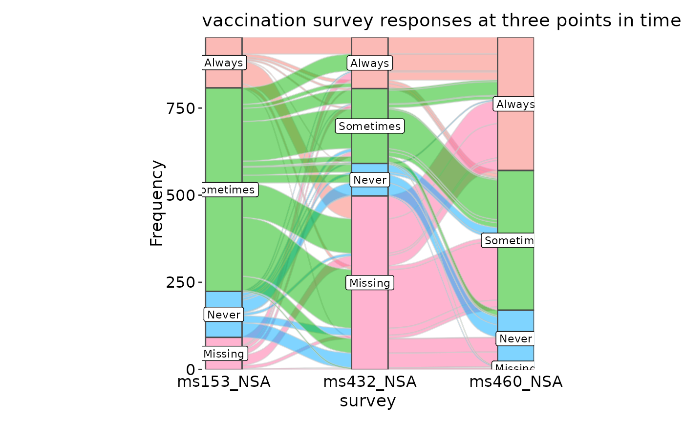
 data(vaccinations, package = "ggalluvial")
vaccinations <- transform(vaccinations,
response = factor(response, rev(levels(response))))
SankeyPlot(vaccinations, x = "survey", stratum = "response", alluvium = "subject",
y = "freq", links_fill_by = "response", nodes_label = TRUE, nodes_alpha = 0.5,
nodes_palette = "seurat", links_palette = "seurat", links_alpha = 0.5,
legend.position = "none", flow = TRUE, expand = c(0, 0, 0, .15), stat = "alluvium",
title = "vaccination survey responses at three points in time")
data(vaccinations, package = "ggalluvial")
vaccinations <- transform(vaccinations,
response = factor(response, rev(levels(response))))
SankeyPlot(vaccinations, x = "survey", stratum = "response", alluvium = "subject",
y = "freq", links_fill_by = "response", nodes_label = TRUE, nodes_alpha = 0.5,
nodes_palette = "seurat", links_palette = "seurat", links_alpha = 0.5,
legend.position = "none", flow = TRUE, expand = c(0, 0, 0, .15), stat = "alluvium",
title = "vaccination survey responses at three points in time")
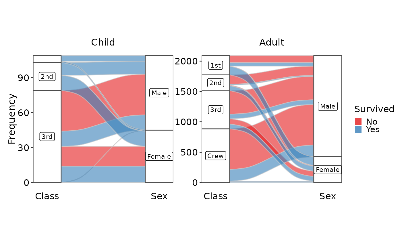
 data(Titanic, package = "datasets")
SankeyPlot(as.data.frame(Titanic), x = c("Class", "Sex"), y = "Freq",
links_fill_by = "Survived", flow = TRUE, facet_by = "Age", facet_scales = "free_y",
nodes_label = TRUE, expand = c(0.05, 0), xlab = "", links_palette = "Set1",
nodes_palcolor = "white", nodes_label_miny = 10)
data(Titanic, package = "datasets")
SankeyPlot(as.data.frame(Titanic), x = c("Class", "Sex"), y = "Freq",
links_fill_by = "Survived", flow = TRUE, facet_by = "Age", facet_scales = "free_y",
nodes_label = TRUE, expand = c(0.05, 0), xlab = "", links_palette = "Set1",
nodes_palcolor = "white", nodes_label_miny = 10)
 # Simulated examples
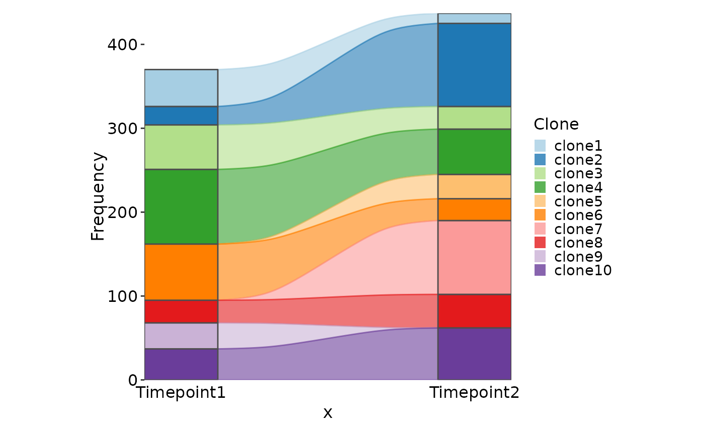
df <- data.frame(
Clone = paste0("clone", 1:10),
Timepoint1 = sample(c(rep(0, 30), 1:100), 10),
Timepoint2 = sample(c(rep(0, 30), 1:100), 10)
)
SankeyPlot(df, x = c("Timepoint1", "Timepoint2"), alluvium = "Clone",
links_color = ".fill")
# Simulated examples
df <- data.frame(
Clone = paste0("clone", 1:10),
Timepoint1 = sample(c(rep(0, 30), 1:100), 10),
Timepoint2 = sample(c(rep(0, 30), 1:100), 10)
)
SankeyPlot(df, x = c("Timepoint1", "Timepoint2"), alluvium = "Clone",
links_color = ".fill")
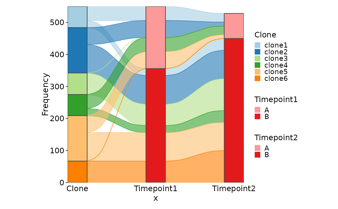
 df <- data.frame(
Clone = rep(paste0("clone", 1:6), each = 2),
Timepoint1 = sample(c(rep(0, 30), 1:100), 6),
Timepoint2 = sample(c(rep(0, 30), 1:100), 6),
Group = rep(c("A", "B"), 6)
)
SankeyPlot(df, x = c(".", "Timepoint1", "Timepoint2"),
stratum = "Group", links_fill_by = "Clone", links_color = ".fill")
df <- data.frame(
Clone = rep(paste0("clone", 1:6), each = 2),
Timepoint1 = sample(c(rep(0, 30), 1:100), 6),
Timepoint2 = sample(c(rep(0, 30), 1:100), 6),
Group = rep(c("A", "B"), 6)
)
SankeyPlot(df, x = c(".", "Timepoint1", "Timepoint2"),
stratum = "Group", links_fill_by = "Clone", links_color = ".fill")
 # }
# }