Basic Design Of The Plots

Color palettes

Available color palettes

The package provides a set of color palettes that are widely used. They are from different packages or used in different tools, including:

• viridis from the viridis package
• brewer.pal.info from the RColorBrewer package
• ggsci_db from the ggsci package
• redmonder.pal.info from the Redmonder package
• metacartocolors from the rcartocolor package
• nord_palettes from the nord package
• The ocean palettes of syspals from the pals package
• colorschemes from the dichromat package
• Some custom palettes including those from jcolors package

All the above palettes are provided by the SCP package. In addition, the SCP package also provides a set of color palettes that are widely used in single-cell analysis, including:

• The discrete colour palettes DiscretePalette from the Seurat package
• scales::hue_pal used by Seurat

See also the following documentation for more details:

• all available color palettes
• show_palettes
• palette_this

Using palette and palcolor arguments to control the colors in the plots

Most plotting functions in plotthis support two arguments to control colors: palette and palcolor. These arguments provide flexible color customization while maintaining consistency with predefined palettes.

The palette argument

The palette argument specifies which predefined color palette to use. You can view all available palettes with show_palettes(). For example:

# Use the "Spectral" palette
BarPlot(data = iris, x = "Species", y = "Petal.Length", palette = "Spectral")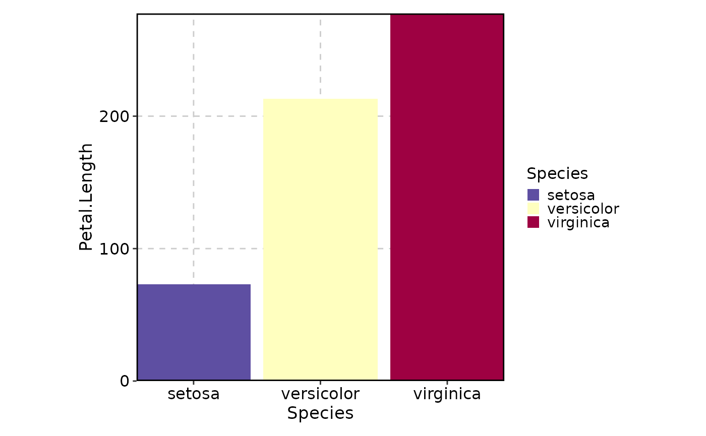

# Use the "nejm" palette from ggsci
BarPlot(data = iris, x = "Species", y = "Petal.Length", palette = "nejm")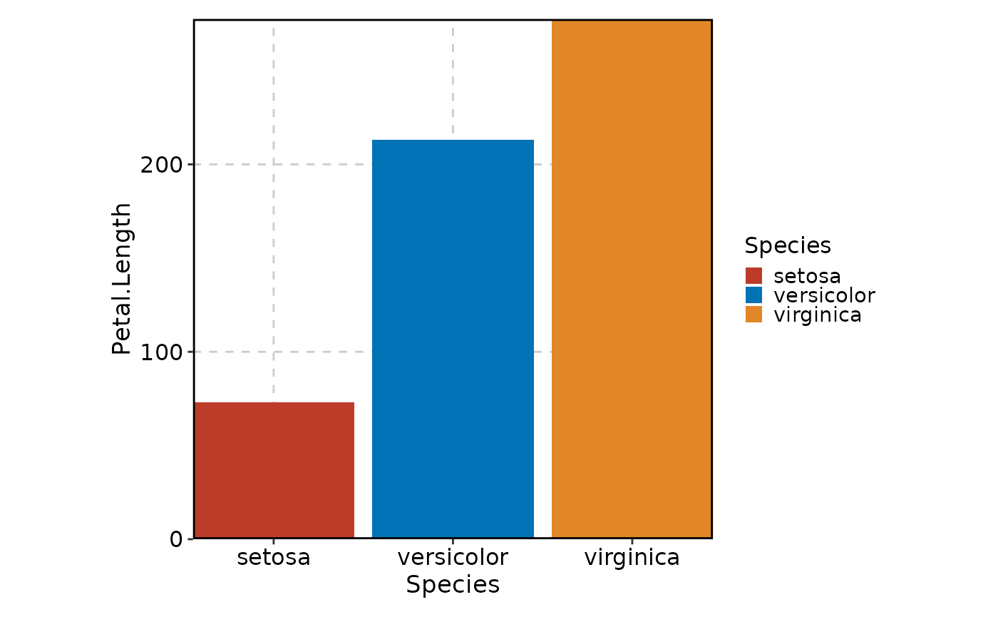

The palette serves as the foundation for color generation. Colors are automatically assigned based on the number of categories or the range of continuous values in your data.

The palcolor argument

The palcolor argument allows you to override specific colors from the palette. The behavior differs for discrete and continuous color scales:

For discrete colors (categorical data)

Use a named vector where names correspond to categories in your data. The function will use the palette as the base and replace only the specified colors:

# Replace specific category colors
BarPlot(
    data = iris,
    x = "Species",
    y = "Petal.Length",
    palette = "Paired",
    palcolor = c("setosa" = "red", "versicolor" = "blue")
)

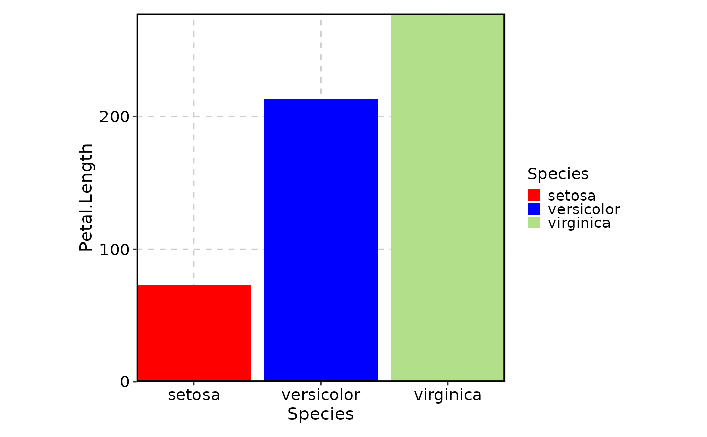
# "virginica" will still use the color from the "Paired" palette

For continuous colors (numeric data)

Use a positional vector where NA values indicate positions to keep from the palette, and non-NA values replace specific positions. The replacement happens evenly distributed across the base palette colors:

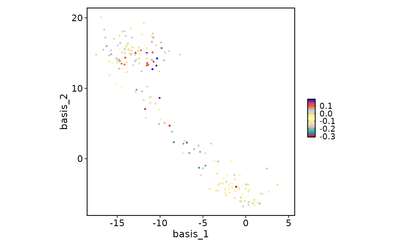
data(dim_example)

FeatureDimPlot(
    data = dim_example,
    features = "stochasticbasis_1",
    palette = "Spectral",
    # The colors will be evenly replace across the palette based on the number of custom colors provided
    # Here are the colors that will be used to generate the ramp colors:
    # "red"       "#3288BD"   "#66C2A5"   "pink"      "#E6F598"   "#FFFFBF"
    # "#FEE08B"   "lightblue" "#F46D43"   "#D53E4F"   "blue"
    # Notice that the 1st, 4th, 8th, and 11th colors in the palette are replaced
    palcolor = c("red", "pink", NA, "lightblue", "blue")
)

The positions are calculated evenly across the palette, so: - With 2 values in palcolor: replaces first and last colors - With 3 values: replaces first, middle, and last colors - With 4 values: replaces at positions 1, 2, 4, and 5 (for a 5-color palette)

This approach ensures smooth color transitions while allowing you to control the endpoints and key intermediate colors.

Customizing NA colors

You can specify the color for NA values using the "NA" key in palcolor**

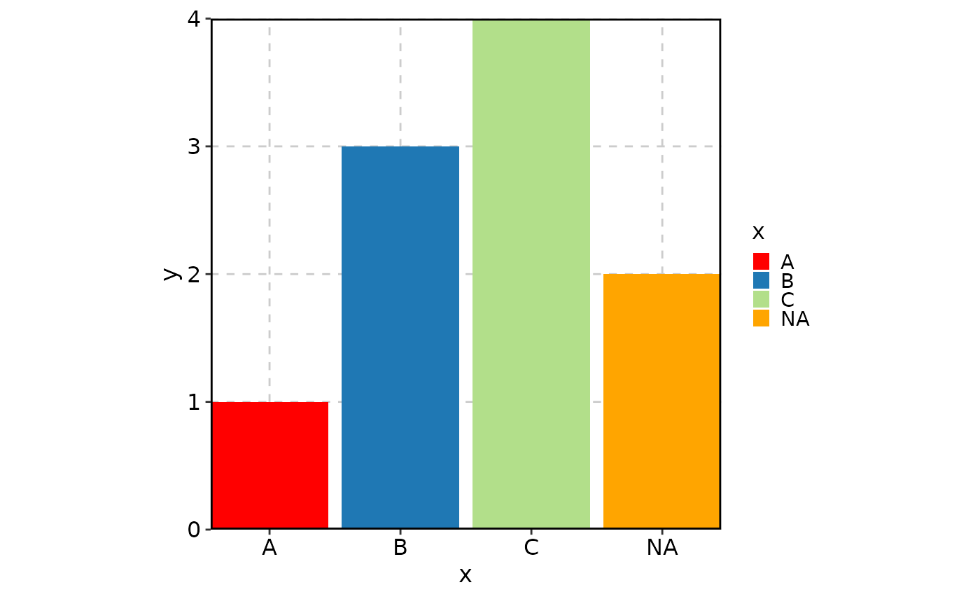
data <- data.frame(x = c("A", NA, "B", "C"), y = c(1, 2, 3, 4))

BarPlot(
    data = data,
    x = "x", y = "y",
    palette = "Paired",
    palcolor = c("A" = "red", "NA" = "orange"),
    # NA values by default will be dropped
    keep_na = TRUE
)

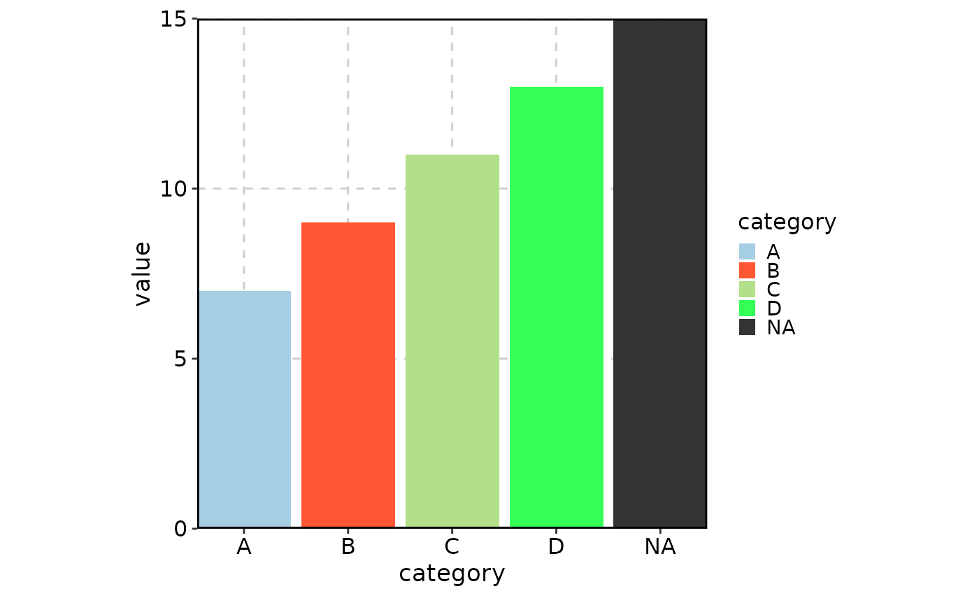
Complete example

Here’s a comprehensive example showing how palette and palcolor work together:

data <- data.frame(
    category = c("A", "B", "C", "D", NA, "A", "B", "C", "D", NA),
    value = c(1, 2, 3, 4, 5, 6, 7, 8, 9, 10)
)

BarPlot(
    data = data,
    x = "category",
    y = "value",
    palette = "Paired",                    # Base palette
    # "A" and "C" will use colors from the "Paired" palette
    palcolor = c(                          # Override specific colors
        "B" = "#FF5733",                   # Custom color for "B"
        "D" = "#33FF57",                   # Custom color for "D"
        "NA" = "#333333"                   # Custom color for NA values
    ),
    keep_na = TRUE                        # Keep NA values in the plot
)

This design gives you fine-grained control over your plot colors while maintaining the convenience of predefined palettes.

Basic implementation of the plotting functions

The plotting functions in plotthis are implemented with the following structure:

SomePlot <- function(
    data,
    # The column to split the data and plot
    # When `facet` is TRUE, the columns specified here will be used to facet the plot
    # When `facet` is FALSE, the columns specified here will be used to split the data
    #   and generate multiple plots and combine them into one
    # If multiple columns are specified
    #   When `facet` is TRUE, up to 2 columns are allowed. If one column,
    #     `ggplot2::facet_wrap` is used, the number of rows and columns is determined
    #     by `nrow` and `ncol`
    #   When `facet` is FALSE, a warning will be issued and the columns will be
    #     concatenated into one column, using `split_by_sep` as the separator
    split_by, split_by_sep,
    # Columns to group the data for plotting
    # For those plotting functions that do not support multiple groups,
    # They will be concatenated into one column, using `group_by_sep` as the separator
    group_by, group_by_sep,
    # Whether to facet the plot, or split the data and combine the plots
    facet, facet_scales,
    # Controls for theming
    theme, theme_args, palette, palcolor, keep_empty, x_text_angle, aspect.ratio,
    legend.position, legend.direction, alpha, title, subtitle, xlab, ylab,
    # The number of rows and columns when `facet_wrap` is used or
    # when `facet` is FALSE, the number of rows and columns to combine the plots
    # For facet_wrap, dir = 'v' will be used when byrow = FALSE
    combine, nrow, ncol, byrow
    # Whether to guess the width and height of the plot in pixels
    # list(plot, width, height) will be returned instead of the plot if TRUE
    seed,
    ...
) {

    # Argument validation

    # Data preparation
    #   Data will be transformed based on the arguments
    #   and split into a list of data frames by split_by

    # Plot for each split data frame
    plots <- lapply(split_data, function(df) {
        # Calling atomic plotting functions to generate the plot
        #   These functions do not need to handle split
        #   All data passed to these functions should feed to the plot
        SomePlotAtomic(df, ...)
    })

    # Combine the plots
    #     patch_work::wrap_plots(plots, nrow, ncol, byrow)
}

Splitting vs faceting

Unlike other plotting packages, plotthis provides a unified interface for both splitting and faceting. For most plots that are created by ggplot2 behind the scenes, plotthis is “facet-aware”.

Most of the plotting functions in plotthis support both splitting and faceting.

The split_by argument is used to split the data and generate multiple plots, and the data in the split_by columns will be used to split the data and generate multiple plots, which will be combined into one plot. Those sub-plots are independent of each other, and they have their own scales and guides. In addition, the split_by_sep argument is used to concatenate the columns specified in split_by into one column, using the specified separator. The palettes/palcolors can be different for each sub-plot using the palette/palcolor argument.

For faceting, the facet_scales argument is used to control the scales of the facets. The facet_wrap function is used when facet_by has one column; otherwise, the facet_grid function is used when facet_by has two columns.

For the plots that do not support faceting (they are not built directly based on ggplot2), the split_by will be a good choice to split the data and generate multiple plots.

Argument naming conventions

The arguments in the plotting functions are named in a consistent way. _ is used to separate words in the argument names, in favor of ., unless the argument is passed to a ggplot2 function (e.g. theme). The _ is used to separate words in the argument names to make the argument names more readable and less confusing with the . in the function names, which could work as a method call. The argument names are all lowercased.

The height and width attributes

All plots created by plotthis come with a height and width attribute. It is an experimental feature that is used to guess the size of the plot in inches. Note that they are NOT the actual size of the plot. They are just a guess based on the elements in the plot.

You can then use these values to set the fig.width and fig.height arguments in the chunk options in R Markdown or options(repr.plot.width = ...) and options(repr.plot.height = ...) in Jupyter notebooks.

You can also use them to save the plot to a file with the guessed size. For example:

p <- SomePlot(x, ...)
png("plot.png", width = attr(p, "width") * 100, height = attr(p, "height") * 100, res = 100)
print(p)
dev.off()

Tracing the ggplot calls for debugging

If a plot is created by ggplot2 behind the scenes, plotthis relies on the gglogger package to trace the ggplot2 calls. The gglogger package is used to log the ggplot2 calls and the arguments passed to the ggplot2 functions. This is useful for debugging and understanding how the plot is created.

options(plotthis.gglogger.enabled = TRUE)

p <- BarPlot(data = iris, x = "Species")

## Registered S3 method overwritten by 'gglogger':
##   method from   
##   +.gg   ggplot2

p$logs

## Reference class object of class "GGLogs"
## Field "logs":
## [[1]]
## Reference class object of class "GGLog"
## Field "code":
## [1] "ggplot2::ggplot(data, aes(x = !!sym(x), y = !!sym(y), fill = !!sym(fill_by)))"
## 
## [[2]]
## Reference class object of class "GGLog"
## Field "code":
## [1] "geom_col(alpha = alpha, width = width, show.legend = TRUE)"
## 
## [[3]]
## Reference class object of class "GGLog"
## Field "code":
## [1] "labs(title = title, subtitle = subtitle, x = xlab %||% x, y = ylab %||% "
## [2] "    y)"                                                                  
## 
## [[4]]
## Reference class object of class "GGLog"
## Field "code":
## [1] "scale_x_discrete(expand = expand$x, drop = !isTRUE(keep_empty_x))"
## 
## [[5]]
## Reference class object of class "GGLog"
## Field "code":
## [1] "scale_y_continuous(expand = expand$y)"
## 
## [[6]]
## Reference class object of class "GGLog"
## Field "code":
## [1] "do.call(theme, theme_args)"
## 
## [[7]]
## Reference class object of class "GGLog"
## Field "code":
## [1] "ggplot2::theme(aspect.ratio = aspect.ratio, legend.position = legend.position, "               
## [2] "    legend.direction = legend.direction, panel.grid.major = element_line(colour = \"grey80\", "
## [3] "        linetype = 2), axis.text.x = element_text(angle = x_text_angle, "                      
## [4] "        hjust = just$h, vjust = just$v))"                                                      
## 
## [[8]]
## Reference class object of class "GGLog"
## Field "code":
## [1] "scale_fill_manual(name = fill_name %||% fill_by, na.value = colors[\"NA\"] %||% "
## [2] "    \"grey80\", values = colors, guide = fill_guide)"                            
## 
## [[9]]
## Reference class object of class "GGLog"
## Field "code":
## [1] "coord_cartesian(ylim = c(y_min, y_max))"

Providing extra data for plotting

When extra data is needed for plotting, plotthis usually provides an argument to receive it. But you can prepare the data and attached as an attribute to the main data frame, and pass @extra to the argument. So the function can access the extra data by attr(data, "extra"). For example:

data <- gsea_result
attr(data, "gene_ranks") <- gene_ranks
attr(data, "gene_sets") <- gene_sets
GSEAPlot(data)

# Equivalent to
GSEAPlot(data, gene_ranks = gene_ranks, gene_sets = gene_sets)

Handling NA values and unused levels of factors

NA values

When NA values appear in the grouping variables or category variables that are used to in the plot (x-axis, fill, color, group, etc.), they will be excluded by default. You can use keep_na option to control whether and how to keep the NA values.

• TRUE: just keep the NA values as they are, and they will be treated as a separate group or category. They will be included in the plot and the legend. The color for the NA values will be grey80 by default, but you can customize it using the palcolor argument (palcolor = list("NA" = "orange")).
• FALSE: drop the NA values, and they will not be included in the plot or the legend. This is the default behavior.
• "missing": or other character string, will replace the NA values with the specified string, and they will be treated as a separate group or category. They will be included in the plot and the legend. The color for the values will be determined by palette and palcolor as usual.

See the above section (Using palette and palcolor arguments to control the colors in the plots) for more details on how to customize the colors for NA values.

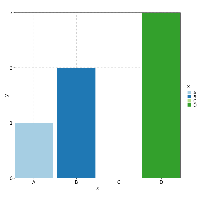
Unused (Empty) levels of factors

When there are unused levels of factors in the grouping variables or category variables that are used to in the plot (x-axis, fill, color, group, etc.), they will be included in the plot by default. You can use keep_empty option to control whether and how to keep the unused levels of factors.

keep_empty can take 3 values:

• TRUE: just keep the unused levels of factors as they are, and they will be treated as separate groups or categories. They will be included in the plot and the legend.
• FALSE: drop the unused levels of factors, and they will not be included in the plot or the legend. This is the default behavior.
• "level" or "levels": The unused levels of factors will not be plotted (for example, on x-axis), but they will be included when determining the colors for the groups or categories, and they will not be included in the legend. Use TRUE if you want to include them in the legend.

When keep_empty is TRUE or "level", the colors for the unused levels of factors will be determined by palette and palcolor as usual, even though they are not plotted (they will affect the colors of existing levels).

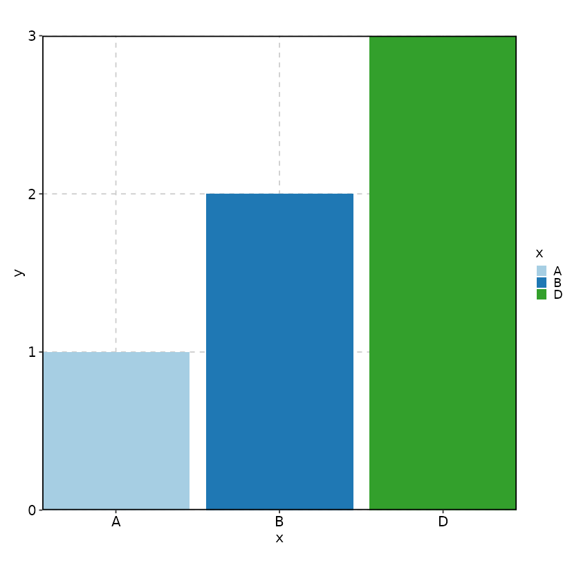
data <- data.frame(
    # C is an unused level
    x = factor(c("A", "B", "D"), levels = c("A", "B", "C", "D")),
    y = c(1, 2, 3)
)

# Excluded by default
BarPlot(
    data = data,
    x = "x", y = "y"
)

# Keep the unused level "C"
BarPlot(
    data = data,
    x = "x", y = "y",
    keep_empty = TRUE
)

# Keep the unused level "C" for color assignment but not plotting
BarPlot(
    data = data,
    x = "x", y = "y",
    keep_empty = "level"
)

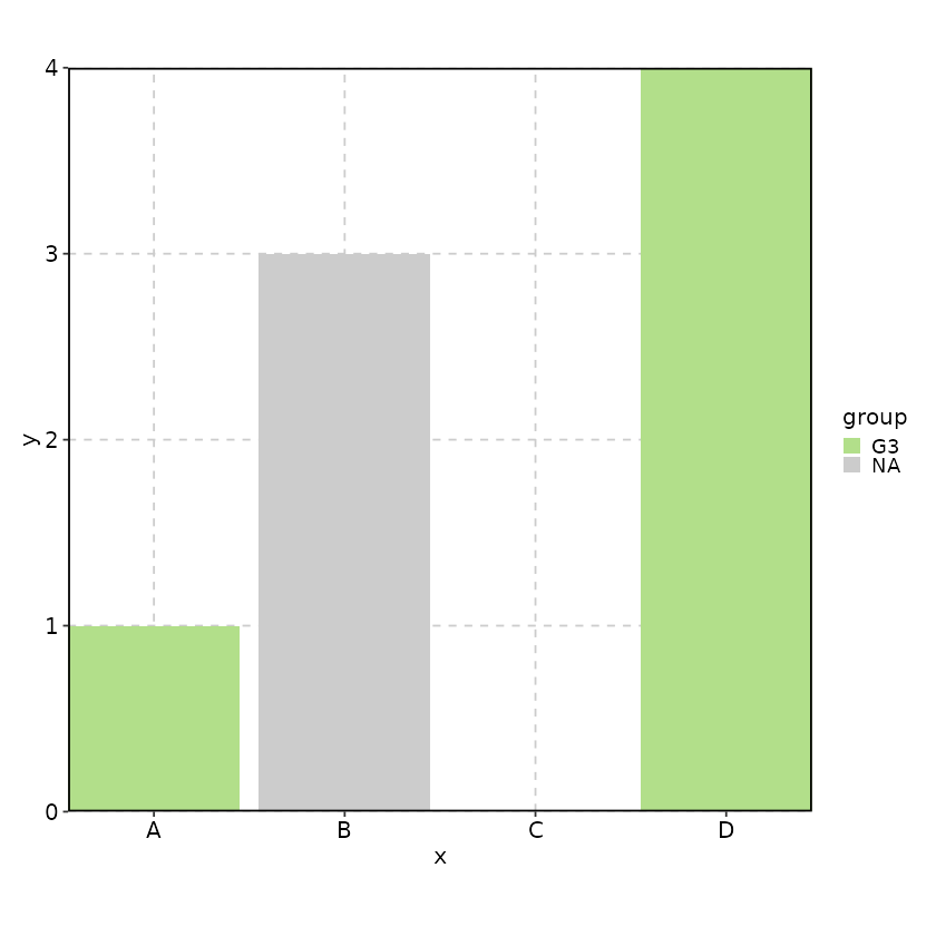
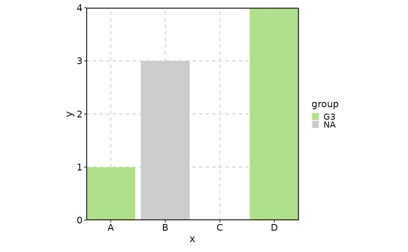
Variable-level control of keeping NA values and unused levels of factors

The keep_na and keep_empty arguments can also take a named list to control the behavior for each variable separately. The names of the list should correspond to the variables in the data. For example:

data <- data.frame(
    x = factor(c("A", NA, "B", "D"), levels = c("A", "B", "C", "D")),
    group = factor(c("G3", "G1", NA, "G3"), levels = c("G1", "G2", "G3")),
    y = c(1, 2, 3, 4)
)

BarPlot(
    data = data,
    x = "x", y = "y", fill_by = "group",
    keep_empty = list(x = TRUE, group = "level"),
    keep_na = list(x = FALSE, group = TRUE)
)