Visualizing data with LLMs
Source:vignettes/Visualizing_data_with_LLMs.Rmd
Visualizing_data_with_LLMs.Rmd
library(scplotter)
api_key_set <- !identical(Sys.getenv("OPENAI_API_KEY"), "")
Introduction
This vignette demonstrates how to use the scplotter
package to visualize data with AI. The package provides a variety of
functions for visualizing single-cell sequencing data, including
scRNA-seq and scTCR-seq/scBCR-seq data.
Setup LLM provider
scplotter uses tidyprompt to provide a
unified interface for different LLM providers. You can set up your
preferred LLM provider using one of the wrappers
provided by tidyprompt.
# Set up LLM provider
provider <- tidyprompt::llm_provider_openai(
    parameters = list(model = "deepseek-v4-flash", stream =
      getOption("tidyprompt.stream", TRUE)),
    verbose = getOption("tidyprompt.verbose", TRUE),
    url = "https://api.deepseek.com/chat/completions",
    api_key = Sys.getenv("OPENAI_API_KEY")
)

chat <- SCPlotterChat$new(provider = provider)
Setup the data for visualization
By default, chat will detects the data used for
visualization from the .GlobalEnv and data exported from
the Seurat, SeuratObject, and
scRepertoire packages.
You can also ask to list the available data:
chat$ask("List the available data that can be used for visualization.")
#>
#> Tool identified:  ListData
#> Available data objects:
#> -  scplotter::cellphonedb_res :  A toy example of CellPhoneDB output from LIANA
#> -  scplotter::ifnb_sub :  A subsetted version of 'ifnb' datasets
#> -  scplotter::pancreas_sub :  A subsetted version of mouse 'pancreas' datasets
#> -  Seurat::cc.genes :  Cell cycle genes
#> -  Seurat::cc.genes.updated.2019 :  Cell cycle genes: 2019 update
#> -  SeuratObject::pbmc_small :  A small example version of the PBMC dataset
#> -  scRepertoire::contig_list :  A list of 8 single-cell T cell receptor sequences runs.
#> -  scRepertoire::mini_contig_list :  Processed subset of 'contig_list'
#> -  scRepertoire::scRep_example :  A Seurat object of 500 single T cells,
# or you can do it explicitly
# chat$list_data()
To set up the data manually, you can use the set_data()
method.
chat$set_data(scplotter::cellphonedb_res)
# To let the LLM to detect the data from the prompt again:
chat$set_data(NULL)
To use your own data, you can either set the data manually or use the
set_data() method or you can load the data in the global
environment and mention it in your prompt.
List the available tools
You can list the available functions by using the
list_tools() method.
chat$list_tools()
#> Available tools:
#> -  gt :  Programmatic clone selection for TCR/BCR repertoire analysis
#>    Clone selectors provide a programmatic, expression-based system for filtering
#>    and selecting T cell and B cell clones from immune repertoire data. They are
#>    the foundation of clone-level analysis in    scplotter   , enabling flexible
#>    clone selection without manual specification of clone IDs.
#>
#>    Clone selectors operate on data frames containing clone abundance information
#>    (clone IDs paired with group-level counts or fractions). They evaluate
#>    selection criteria — such as abundance thresholds, group comparisons, or
#>    shared presence across conditions — and return either the selected clone IDs,
#>    a logical indicator vector, or a filtered data frame. The system is
#>    context-aware: it automatically detects whether it is being called from
#>    within a    dplyr    pipeline, a    scplotter    function, or standalone
#>    code, and adjusts its default behavior accordingly.
#>
#>    The following selector functions are available:
#>
#>        top()    — select the    n    largest clones by abundance
#>        sel()    — select clones matching a custom logical expression
#>        uniq()    — select clones unique to a specified group
#>        shared()    — select clones present in all specified groups
#>        gt()   ,    ge()   ,    lt()   ,    le()   ,    eq()   ,    ne()    — comparison-based selection
#>        and()   ,    or()    — combine multiple selector results
#>
#> -  CellDimPlot :  Cell Dimension Reduction Plot
#>    Visualizes single-cell data in reduced dimension space (e.g., UMAP, t-SNE,
#>    PCA). This is the primary function for exploring cell clustering, cell
#>    identity, and spatial relationships in transcriptomics datasets. It creates
#>    scatter plots where each point represents a cell, positioned by its
#>    coordinates in the reduced dimension space and colored by metadata variables
#>    such as cell type, sample condition, or cluster assignment.
#>
#>    CellDimPlot    serves as a unified interface across multiple single-cell data
#>    containers:
#>
#>        Seurat objects    — Extracts embeddings from    Reductions()    and
#>    metadata from    @meta.data   . The default reduction is auto-detected
#>    via    default_dimreduc()   .
#>        Giotto objects    — Extracts spatial dimension reductions and cell
#>    metadata using    spat_unit    and    feat_type    to identify the correct
#>    spatial unit and feature type.
#>        h5ad files    (.h5ad or opened    H5File   ) — Reads from    obsm    for
#>    embeddings and    obs    for metadata. Reduction names are automatically
#>    prefixed with    "X_"    when needed (e.g.,    "umap"    →    "X_umap"   ).
#>
#>
#>    Beyond basic cluster visualization,    CellDimPlot    supports a rich set of
#>    visual overlays and analytical enhancements:
#>
#>        Cluster highlighting    — Emphasize cells matching a logical
#>    expression while dimming others (   highlight   ).
#>        Group labels    — Add text labels at group centroids (   label   ,
#>    label_insitu   ).
#>        Group marks    — Draw boundary shapes around groups: ellipse,
#>    rectangle, or circle (   add_mark   ,    mark_type   ).
#>        Density contours    — Overlay 2D density estimates (   add_density   ).
#>        Neighbor graphs    — Draw edges between neighboring cells from
#>    k-NN or shared-nearest-neighbor graphs (   graph   ).
#>        Lineage trajectories    — Overlay pseudotime lineage curves
#>    (   lineages   ).
#>        Velocity arrows    — Overlay RNA velocity vectors on the embedding
#>    (   velocity   ). For dedicated velocity visualization with grid or
#>    stream plots, see    CellVelocityPlot   .
#>        Statistical charts    — Embed small bar, ring, or line charts at
#>    group positions showing composition of a second variable (   stat_by   ,
#>    stat_plot_type   ).
#>        Hexagonal binning    — Replace scatter points with binned hexagons
#>    for large datasets (   hex   ).
#>        3D visualization    — Plot three dimensions by specifying
#>    dims = 1:3   .
#>        Rasterization    — Render points as a raster image for performance
#>    with large cell counts (   raster   ).
#>
#> -  ClonalVolumePlot :  Clonal Volume Plot
#>    Visualizes the number (or fraction) of unique T-cell or B-cell clones across
#>    samples and metadata groups. Clonal volume — the count of distinct clonotypes
#>    detected in a sample — is a fundamental measure of immune repertoire diversity.
#>    Higher clonal volume indicates a more diverse repertoire, while lower volume
#>    may reflect clonal expansion in response to antigen stimulation.
#>
#>    ClonalVolumePlot    computes clonal counts via
#>    scRepertoire::clonalQuant()    and
#>    visualizes them as bar, box, or violin plots. It accepts both
#>    scRepertoire    combined TCR/BCR data and Seurat objects with clonal
#>    information integrated via    scRepertoire::combineExpression()   .
#> -  ClonalRarefactionPlot :  Clonal Rarefaction Plot
#>    Visualizes clonal rarefaction curves — estimates of clone richness as a
#>    function of sampling depth. Rarefaction addresses a fundamental challenge
#>    in immune repertoire analysis: the number of clones observed depends on
#>    how many cells are sequenced. By repeatedly subsampling (bootstrapping)
#>    the data at varying depths, rarefaction curves reveal whether the
#>    repertoire has been sampled to saturation or whether additional
#>    sequencing would uncover many more clones.
#>
#>    ClonalRarefactionPlot    extracts clone count data from the repertoire,
#>    optionally groups it by metadata columns, and generates rarefaction
#>    curves via    plotthis::RarefactionPlot()   .
#>    When    split_by    is specified, separate plots are generated for each split
#>    group and combined into a multi-panel layout.
#> -  ClonalStatPlot :  Visualize clone abundance, frequency, and dynamics across groups
#>    ClonalStatPlot provides a unified interface for visualizing the abundance, frequency,
#>    and dynamics of T cell and B cell clones across experimental groups. It is the most
#>    versatile clone visualization function in scplotter, offering multiple plot types
#>    for different analytical purposes.
#>
#>    The function operates on the output of    scRepertoire::combineTCR()   ,
#>    scRepertoire::combineBCR()   , or
#>    scRepertoire::combineExpression()   . Clones are
#>    identified by their CDR3 amino acid sequence, nucleotide sequence, V(D)J gene usage,
#>    or a combination thereof (via    clone_call   ). The function then computes clone-level
#>    statistics (size, fraction, or count of clones) within each group and renders them
#>    using one of ten supported plot types.
#>
#>    A defining feature of ClonalStatPlot is its flexible clone selection system. Clones
#>    can be specified directly by their IDs, or selected programmatically using expression
#>    selectors such as    top()   ,    sel()   ,    shared()   ,    uniq()   , and
#>    comparison operators (   gt()   ,    lt()   ,    eq()   , etc.). These selectors
#>    evaluate within the context of each faceting/splitting group, enabling per-group
#>    selection of the most expanded clones, clones shared between conditions, or clones
#>    meeting custom abundance thresholds. See the    Clone selection    section below
#>    and    CloneSelectors    for full details.
#>
#>    Clones can also be aggregated into named groups (by passing a named list to
#>    clones   ), where each group is defined by its own selection expression. In
#>    this mode, the visualization unit becomes the clone group rather than individual
#>    clones, enabling comparisons such as "hyper-expanded clones in condition A" vs.
#>    "hyper-expanded clones in condition B."
#> -  ClonalCompositionPlot :  Clonal Composition Plot
#>    Visualizes the composition of the immune repertoire by categorizing clones
#>    into abundance groups (Rare, Small, Medium, Large, Hyperexpanded) and
#>    plotting their relative proportions across samples or metadata groups.
#>    This reveals the overall structure of the repertoire — whether it is
#>    dominated by a few large clones (clonal expansion) or composed of many
#>    small clones (high diversity).
#>
#>    ClonalCompositionPlot    supports three analysis methods:
#>
#>        Homeostasis    (   "homeostasis"   ,    "homeo"   ,    "rel"   ) —
#>    Clones are binned by their frequency (fraction of the total
#>    repertoire) into categories such as Rare, Small, Medium, Large,
#>    and Hyperexpanded. Uses
#>    scRepertoire::clonalHomeostasis()   .
#>        Top clones    (   "top"   ) — Clones are ranked and binned by
#>    their rank index (e.g., top 10, top 100, etc.). Uses
#>    scRepertoire::clonalProportion()   .
#>        Rare clones    (   "rare"   ) — Clones are binned by their
#>    absolute size (clone count). Uses clone size thresholds directly.
#>
#> -  EnrichmentPlot :  Visualize gene set enrichment and over-representation analysis results
#>    Gene set enrichment analysis identifies biological pathways, gene ontologies,
#>    or functional categories that are statistically over-represented among a list
#>    of genes of interest (e.g., differentially expressed genes from a single-cell
#>    RNA-seq experiment). Rather than interpreting individual genes in isolation,
#>    enrichment analysis places gene-level results into a broader biological context,
#>    revealing which processes, functions, or diseases are perturbed.
#>
#>    EnrichmentPlot    generates publication-quality visualizations for enrichment
#>    results across eight distinct plot types, each suited to a different analytical
#>    perspective:
#>
#>        bar    — Horizontal bar chart of the top enriched terms, ordered by
#>    significance. Best for a quick overview or when showing a small number of terms.
#>        dot    — Dot plot where x-axis shows a continuous metric (default:
#>    GeneRatio   ), dot size reflects gene count, and dot color reflects
#>    significance. Ideal for comparing terms along two dimensions simultaneously.
#>        lollipop    — Lollipop chart combining dot and bar aesthetics.
#>    Similar to the dot plot but with stems emphasizing the ranking.
#>        comparison    — Side-by-side dot plot comparing enrichment across
#>    groups (e.g., cell types, conditions). Requires    group_by   .
#>        network    — Network visualization where nodes are enriched terms
#>    and edges represent overlapping gene sets. Reveals functional modules and
#>    redundant terms.
#>        enrichmap    — Enrichment map similar to the network plot but
#>    optimized for large term sets (default    top_term = 100   ). Nodes are
#>    terms and edges represent gene overlap.
#>        wordcloud    — Word cloud where term size reflects significance.
#>    Can display either enrichment terms (   word_type = "term"   ) or
#>    individual gene symbols (   word_type = "feature"   ).
#>        heatmap    — Heatmap of enrichment significance across groups
#>    (   group_by    is mapped to columns). Useful for comparing enrichment
#>    patterns across multiple conditions or cell types.
#>
#>
#>    The function auto-detects the input data format (   clusterProfiler    or
#>    enrichR   ) and delegates visualization to the appropriate    plotthis
#>    plotting function.
#> -  eq :  Programmatic clone selection for TCR/BCR repertoire analysis
#>    Clone selectors provide a programmatic, expression-based system for filtering
#>    and selecting T cell and B cell clones from immune repertoire data. They are
#>    the foundation of clone-level analysis in    scplotter   , enabling flexible
#>    clone selection without manual specification of clone IDs.
#>
#>    Clone selectors operate on data frames containing clone abundance information
#>    (clone IDs paired with group-level counts or fractions). They evaluate
#>    selection criteria — such as abundance thresholds, group comparisons, or
#>    shared presence across conditions — and return either the selected clone IDs,
#>    a logical indicator vector, or a filtered data frame. The system is
#>    context-aware: it automatically detects whether it is being called from
#>    within a    dplyr    pipeline, a    scplotter    function, or standalone
#>    code, and adjusts its default behavior accordingly.
#>
#>    The following selector functions are available:
#>
#>        top()    — select the    n    largest clones by abundance
#>        sel()    — select clones matching a custom logical expression
#>        uniq()    — select clones unique to a specified group
#>        shared()    — select clones present in all specified groups
#>        gt()   ,    ge()   ,    lt()   ,    le()   ,    eq()   ,    ne()    — comparison-based selection
#>        and()   ,    or()    — combine multiple selector results
#>
#> -  CellVelocityPlot :  Cell Velocity Plot
#>    Visualizes RNA velocity on a reduced-dimension embedding. RNA velocity
#>    infers the future transcriptional state of individual cells by modeling the
#>    ratio of unspliced (nascent) to spliced (mature) mRNA transcripts. On a
#>    dimension reduction plot, velocity is displayed as arrows (or grid/stream
#>    fields) showing the predicted direction and magnitude of transcriptional
#>    change for each cell — effectively revealing the "flow" of cells through
#>    differentiation, development, or other state transitions.
#>
#>    CellVelocityPlot    serves as a unified interface across multiple single-cell
#>    data containers:
#>
#>        Seurat objects    — Extracts embeddings from both the main
#>    reduction (   reduction   ) and the velocity reduction
#>    (   v_reduction   ) via    Embeddings()   ; metadata for grouping via
#>    @meta.data   .
#>        Giotto objects    — Extracts dimension reductions via
#>    getDimReduction()    using    spat_unit    and    feat_type    to identify
#>    the correct spatial unit and feature type.
#>        h5ad files    (.h5ad or opened    H5File   ) — Reads from    obsm    for
#>    both the main and velocity embeddings;    obs    for metadata. Reduction
#>    names are automatically prefixed with    "X_"    when needed.
#>
#> -  SpatFeaturePlot :  Visualize feature expression on spatial coordinates
#>    Plot continuous feature values — gene expression, dimension reduction
#>    components, metadata columns, or any numeric variable — directly on
#>    spatial tissue coordinates.    SpatFeaturePlot()    is the spatial
#>    analogue of a feature plot over a UMAP/t-SNE embedding: it paints each
#>    spot, cell, or molecule with the expression level of one or more features,
#>    revealing the spatial organization of gene activity.
#>
#>    Multiple features are automatically faceted, making it easy to compare
#>    spatial expression patterns across a gene panel in a single plot. For
#>    categorical grouping (e.g., cluster identity on spatial coordinates), use
#>    SpatDimPlot    instead.
#> -  shared :  Programmatic clone selection for TCR/BCR repertoire analysis
#>    Clone selectors provide a programmatic, expression-based system for filtering
#>    and selecting T cell and B cell clones from immune repertoire data. They are
#>    the foundation of clone-level analysis in    scplotter   , enabling flexible
#>    clone selection without manual specification of clone IDs.
#>
#>    Clone selectors operate on data frames containing clone abundance information
#>    (clone IDs paired with group-level counts or fractions). They evaluate
#>    selection criteria — such as abundance thresholds, group comparisons, or
#>    shared presence across conditions — and return either the selected clone IDs,
#>    a logical indicator vector, or a filtered data frame. The system is
#>    context-aware: it automatically detects whether it is being called from
#>    within a    dplyr    pipeline, a    scplotter    function, or standalone
#>    code, and adjusts its default behavior accordingly.
#>
#>    The following selector functions are available:
#>
#>        top()    — select the    n    largest clones by abundance
#>        sel()    — select clones matching a custom logical expression
#>        uniq()    — select clones unique to a specified group
#>        shared()    — select clones present in all specified groups
#>        gt()   ,    ge()   ,    lt()   ,    le()   ,    eq()   ,    ne()    — comparison-based selection
#>        and()   ,    or()    — combine multiple selector results
#>
#> -  CellStatPlot :  Cell statistics plot
#>    Visualizes cell-level statistics — counts, fractions, and composition —
#>    across cell identities and metadata groupings. This is the primary function
#>    for exploring the distribution of cell types, clusters, and categorical
#>    metadata in single-cell transcriptomics datasets. It answers questions such
#>    as: "What proportion of each cell type is in each condition?", "How do
#>    cluster abundances change across samples?", and "What is the clonal
#>    composition within each cell type?"
#>
#>    CellStatPlot    serves as a unified interface across 15+ visualization
#>    types, all driven by a common data aggregation and fraction-calculation
#>    pipeline. It supports four single-cell data containers:
#>
#>        Seurat objects    — Extracts    @meta.data   ; uses    Idents()    as
#>    the default identity when    ident = NULL   .
#>        Giotto objects    — Extracts cell metadata via
#>    getCellMetadata()    using    spat_unit    and    feat_type   .
#>        h5ad files    (.h5ad or opened    H5File   ) — Reads from    obs
#>    via    h5group_to_dataframe()   .
#>        Data frames    — Internal method; all other methods ultimately
#>    delegate here after metadata extraction.
#>
#> -  ne :  Programmatic clone selection for TCR/BCR repertoire analysis
#>    Clone selectors provide a programmatic, expression-based system for filtering
#>    and selecting T cell and B cell clones from immune repertoire data. They are
#>    the foundation of clone-level analysis in    scplotter   , enabling flexible
#>    clone selection without manual specification of clone IDs.
#>
#>    Clone selectors operate on data frames containing clone abundance information
#>    (clone IDs paired with group-level counts or fractions). They evaluate
#>    selection criteria — such as abundance thresholds, group comparisons, or
#>    shared presence across conditions — and return either the selected clone IDs,
#>    a logical indicator vector, or a filtered data frame. The system is
#>    context-aware: it automatically detects whether it is being called from
#>    within a    dplyr    pipeline, a    scplotter    function, or standalone
#>    code, and adjusts its default behavior accordingly.
#>
#>    The following selector functions are available:
#>
#>        top()    — select the    n    largest clones by abundance
#>        sel()    — select clones matching a custom logical expression
#>        uniq()    — select clones unique to a specified group
#>        shared()    — select clones present in all specified groups
#>        gt()   ,    ge()   ,    lt()   ,    le()   ,    eq()   ,    ne()    — comparison-based selection
#>        and()   ,    or()    — combine multiple selector results
#>
#> -  SpatDimPlot :  Visualize categorical groups on spatial coordinates
#>    Plot categorical metadata — cluster identities, tissue regions, sample
#>    labels, or any discrete grouping variable — directly on spatial tissue
#>    coordinates.    SpatDimPlot()    is the spatial analogue of a UMAP/t-SNE
#>    plot colored by cluster: each spot, cell, or molecule is colored by its
#>    group membership, making it easy to assess the spatial organization of
#>    cell types, anatomical regions, or experimental conditions.
#>
#>    For continuous features (gene expression, dimension reduction scores),
#>    use    SpatFeaturePlot    instead.
#> -  GSEASummaryPlot :  Objects exported from other packages
#>    These objects are imported from other packages. Follow the links
#>    below to see their documentation.
#>
#>
#>         plotthis   GSEAPlot()   ,    GSEASummaryPlot()
#> -  CCCPlot :  Visualize Cell-Cell Communication (CCC) Interactions
#>    Cell-cell communication (CCC) is the process by which cells send and receive
#>    molecular signals — typically through ligand-receptor (LR) interactions — to
#>    coordinate tissue function. CCC analysis infers these interactions from
#>    single-cell transcriptomics data by identifying which ligand-receptor pairs
#>    are expressed between which cell types, often scoring each interaction by
#>    its magnitude (e.g., expression level, interaction score) and specificity
#>    (e.g., a p-value quantifying how cell-type-specific the interaction is).
#>
#>    CCCPlot    provides a unified interface to visualize CCC inference results
#>    (from tools like CellPhoneDB, LIANA, CellChat, NicheNet, etc.) across many
#>    plot types. It supports two fundamental modes:
#>
#>    Aggregation mode    (   method = "aggregation"   , the default): Ligand-receptor
#>    pairs are aggregated per source-target cell type pair. This shows    which
#>    cell types communicate    and how strongly. Supported plot types:    "network"   ,
#>    "chord"   /   "circos"   ,    "heatmap"   ,    "sankey"   /   "alluvial"   ,    "dot"   .
#>
#>    Interaction mode    (   method = "interaction"   ): Individual ligand-receptor
#>    pairs are plotted. This shows    which specific LR pairs    mediate the
#>    communication. Supported plot types:    "dot"   ,    "network"   ,    "heatmap"   ,
#>    "box"   ,    "violin"   ,    "ridge"   .
#>
#>    The    "linkedheatmap"    plot type is a special case: it does not use the
#>    method    parameter. It displays a side-by-side heatmap where the left side
#>    shows ligand expression across source cell types and the right side shows
#>    receptor expression across target cell types, with links between them
#>    representing the LR pairs. This plot type requires    ligand_means    and
#>    receptor_means    columns.
#>
#>    Under the hood,    CCCPlot    preprocesses the data (aggregating or
#>    reformatting as needed) and delegates rendering to the corresponding
#>    plotthis    package function. All styling and layout arguments accepted by
#>    those functions can be passed through    ...   .
#> -  ClonalResidencyPlot :  Clonal Residency Plot
#>    Visualizes the sharing (residency) of T-cell or B-cell clones across
#>    different samples or metadata groups. Clonal residency analysis reveals
#>    how clonotypes are distributed — whether a clone is private to one
#>    condition or shared across multiple conditions — which is critical for
#>    understanding immune responses, tracking antigen-specific clones, and
#>    identifying public vs. private repertoires.
#>
#>    ClonalResidencyPlot    supports three visualization modes:
#>
#>        Scatter plot    — Compares clone sizes between two groups on
#>    log-transformed axes. Points are colored by clonal category:
#>    singletons (unique to one group), expanded clones, and dual
#>    clones (shared between groups). Correlation statistics are
#>    displayed in the subtitle.
#>        Venn diagram    — Shows the overlap of clone sets between up
#>    to 4 groups. When    with_class = TRUE   , labels include singlet
#>    counts.
#>        UpSet plot    — Shows intersection sizes for any number of
#>    groups. When    with_class = TRUE   , clone classes (singlet,
#>    expanded) are displayed as separate intersections.
#>
#> -  ClustreePlot :  Visualize cluster stability across clustering resolutions
#>    A clustree plot visualizes how cells move between clusters when clustering is
#>    performed at different resolutions. Each resolution level is a column of nodes,
#>    and edges show the flow of cells between clusters at adjacent resolutions.
#>    This is an essential diagnostic for single-cell analysis, helping researchers
#>    choose an appropriate clustering resolution by revealing which clusters are
#>    stable (persistent across resolutions) and which are transient (appear only at
#>    specific resolutions).
#>
#>    This function is a wrapper around    plotthis::ClustreePlot()
#>    that automatically extracts the metadata from Seurat objects. For data frames,
#>    the data is passed directly to    plotthis   .
#> -  ClonalKmerPlot :  Visualize CDR3 k-mer (motif) frequency
#>    Short amino acid motifs within CDR3 sequences — termed    k-mers    — can reveal
#>    shared binding specificities, common structural elements, and repertoire-level
#>    sequence features that are not apparent from full-length sequence analysis
#>    alone. Specific k-mers may be enriched in responses to particular antigens,
#>    represent public TCR/BCR motifs shared across individuals, or reflect
#>    convergent recombination events.
#> -  ClonalPositionalPlot :  Visualize positional properties of CDR3 sequences
#>    The complementarity-determining region 3 (CDR3) is the most variable region of
#>    T cell and B cell receptors, and is the primary determinant of antigen
#>    specificity. Analyzing how amino acid composition, diversity, and
#>    physicochemical properties vary across CDR3 positions provides insight into
#>    repertoire structure, selection pressures, and the biophysical constraints
#>    that shape antigen recognition.
#> -  uniq :  Programmatic clone selection for TCR/BCR repertoire analysis
#>    Clone selectors provide a programmatic, expression-based system for filtering
#>    and selecting T cell and B cell clones from immune repertoire data. They are
#>    the foundation of clone-level analysis in    scplotter   , enabling flexible
#>    clone selection without manual specification of clone IDs.
#>
#>    Clone selectors operate on data frames containing clone abundance information
#>    (clone IDs paired with group-level counts or fractions). They evaluate
#>    selection criteria — such as abundance thresholds, group comparisons, or
#>    shared presence across conditions — and return either the selected clone IDs,
#>    a logical indicator vector, or a filtered data frame. The system is
#>    context-aware: it automatically detects whether it is being called from
#>    within a    dplyr    pipeline, a    scplotter    function, or standalone
#>    code, and adjusts its default behavior accordingly.
#>
#>    The following selector functions are available:
#>
#>        top()    — select the    n    largest clones by abundance
#>        sel()    — select clones matching a custom logical expression
#>        uniq()    — select clones unique to a specified group
#>        shared()    — select clones present in all specified groups
#>        gt()   ,    ge()   ,    lt()   ,    le()   ,    eq()   ,    ne()    — comparison-based selection
#>        and()   ,    or()    — combine multiple selector results
#>
#> -  top :  Programmatic clone selection for TCR/BCR repertoire analysis
#>    Clone selectors provide a programmatic, expression-based system for filtering
#>    and selecting T cell and B cell clones from immune repertoire data. They are
#>    the foundation of clone-level analysis in    scplotter   , enabling flexible
#>    clone selection without manual specification of clone IDs.
#>
#>    Clone selectors operate on data frames containing clone abundance information
#>    (clone IDs paired with group-level counts or fractions). They evaluate
#>    selection criteria — such as abundance thresholds, group comparisons, or
#>    shared presence across conditions — and return either the selected clone IDs,
#>    a logical indicator vector, or a filtered data frame. The system is
#>    context-aware: it automatically detects whether it is being called from
#>    within a    dplyr    pipeline, a    scplotter    function, or standalone
#>    code, and adjusts its default behavior accordingly.
#>
#>    The following selector functions are available:
#>
#>        top()    — select the    n    largest clones by abundance
#>        sel()    — select clones matching a custom logical expression
#>        uniq()    — select clones unique to a specified group
#>        shared()    — select clones present in all specified groups
#>        gt()   ,    ge()   ,    lt()   ,    le()   ,    eq()   ,    ne()    — comparison-based selection
#>        and()   ,    or()    — combine multiple selector results
#>
#> -  le :  Programmatic clone selection for TCR/BCR repertoire analysis
#>    Clone selectors provide a programmatic, expression-based system for filtering
#>    and selecting T cell and B cell clones from immune repertoire data. They are
#>    the foundation of clone-level analysis in    scplotter   , enabling flexible
#>    clone selection without manual specification of clone IDs.
#>
#>    Clone selectors operate on data frames containing clone abundance information
#>    (clone IDs paired with group-level counts or fractions). They evaluate
#>    selection criteria — such as abundance thresholds, group comparisons, or
#>    shared presence across conditions — and return either the selected clone IDs,
#>    a logical indicator vector, or a filtered data frame. The system is
#>    context-aware: it automatically detects whether it is being called from
#>    within a    dplyr    pipeline, a    scplotter    function, or standalone
#>    code, and adjusts its default behavior accordingly.
#>
#>    The following selector functions are available:
#>
#>        top()    — select the    n    largest clones by abundance
#>        sel()    — select clones matching a custom logical expression
#>        uniq()    — select clones unique to a specified group
#>        shared()    — select clones present in all specified groups
#>        gt()   ,    ge()   ,    lt()   ,    le()   ,    eq()   ,    ne()    — comparison-based selection
#>        and()   ,    or()    — combine multiple selector results
#>
#> -  MarkersPlot :  Visualize differential expression markers
#>    Visualize differential expression (DE) results — typically the output of
#>    Seurat::FindMarkers()    or
#>    Seurat::FindAllMarkers()    — across a
#>    variety of plot types. You can also compose the DE results from other
#>    tools into a data frame with the required columns and use this function to visualize them.
#>
#>    MarkersPlot()    bridges the gap between DE
#>    testing and visualization by providing a unified interface for both
#>    summary-level DE visualizations    (volcano, jitter, heatmap, and dot
#>    plots of fold changes and significance) and    expression-level
#>    visualizations    (violin, box, bar, ridge, heatmap, and dot plots of actual
#>    expression values from a Seurat object).
#>
#>    The function handles two broad categories of plots:
#>
#>        DE summary plots    (no    object    required): visualize the
#>    DE statistics themselves — log2 fold change, percentage difference,
#>    p-values, and adjusted p-values — across groups or comparisons.
#>
#>        "volcano"    /    "volcano_log2fc"    — Volcano plot with
#>    log2 fold change on the x-axis and    -log_{10}(p)    on the y-axis.
#>    Genes passing the    cutoff    are highlighted and top genes are
#>    labeled. Ideal for overview of effect size vs. significance.
#>        "volcano_pct"    — Volcano plot with percentage-point
#>    difference (   pct.1 - pct.2   ) on the x-axis. Useful when the
#>    biological question is about detection rate rather than expression
#>    magnitude.
#>        "jitter"    /    "jitter_log2fc"    — Jitter plot of log2
#>    fold changes across groups (defined by    each   ). Dot size
#>    encodes    -log_{10}(p)   . Reveals distribution of effect sizes
#>    per cluster or condition.
#>        "jitter_pct"    — Jitter plot of percentage-point
#>    differences across groups.
#>        "heatmap_log2fc"    — Heatmap of log2 fold changes (genes
#>    × groups). Cells can be marked for significance via    cutoff
#>    and    sig_mark   .
#>        "heatmap_pct"    — Heatmap of percentage-point differences
#>    (genes × groups). Same significance-marking support.
#>        "dot_log2fc"    — Dot plot of log2 fold changes (genes ×
#>    groups). Dot size encodes    -log_{10}(p)   .
#>        "dot_pct"    — Dot plot of percentage-point differences
#>    (genes × groups). Dot size encodes    -log_{10}(p)   .
#>
#>        Expression plots    (   object    required): visualize the
#>    actual expression values of the selected marker genes in the context of
#>    the original Seurat object. These are useful for validating DE results
#>    by inspecting the underlying expression distributions.
#>
#>        "heatmap"    — Expression heatmap of selected marker genes.
#>        "violin"    — Violin plots of expression per gene.
#>        "box"    — Box plots of expression per gene.
#>        "bar"    — Bar plots of mean expression per gene.
#>        "ridge"    — Ridge plots of expression distribution per gene.
#>        "dot"    — Dot plot of expression (fraction expressing ×
#>    mean expression) per gene.
#>
#>
#> -  ClonalOverlapPlot :  Clonal Overlap Plot
#>    Visualizes the overlap (sharing) of T-cell or B-cell clonotypes between
#>    samples or metadata groups as a heatmap. Each cell in the heatmap
#>    quantifies the degree of clonal sharing between two groups, using one of
#>    several similarity or overlap metrics. This is a key analysis for
#>    identifying public clones shared across individuals, tracking
#>    antigen-specific clones across time points or tissues, and comparing
#>    repertoire similarity between conditions.
#>
#>    ClonalOverlapPlot    computes pairwise overlap via
#>    scRepertoire::clonalOverlap()
#>    and visualizes the resulting matrix as a labeled heatmap using
#>    plotthis::Heatmap()   .
#> -  ge :  Programmatic clone selection for TCR/BCR repertoire analysis
#>    Clone selectors provide a programmatic, expression-based system for filtering
#>    and selecting T cell and B cell clones from immune repertoire data. They are
#>    the foundation of clone-level analysis in    scplotter   , enabling flexible
#>    clone selection without manual specification of clone IDs.
#>
#>    Clone selectors operate on data frames containing clone abundance information
#>    (clone IDs paired with group-level counts or fractions). They evaluate
#>    selection criteria — such as abundance thresholds, group comparisons, or
#>    shared presence across conditions — and return either the selected clone IDs,
#>    a logical indicator vector, or a filtered data frame. The system is
#>    context-aware: it automatically detects whether it is being called from
#>    within a    dplyr    pipeline, a    scplotter    function, or standalone
#>    code, and adjusts its default behavior accordingly.
#>
#>    The following selector functions are available:
#>
#>        top()    — select the    n    largest clones by abundance
#>        sel()    — select clones matching a custom logical expression
#>        uniq()    — select clones unique to a specified group
#>        shared()    — select clones present in all specified groups
#>        gt()   ,    ge()   ,    lt()   ,    le()   ,    eq()   ,    ne()    — comparison-based selection
#>        and()   ,    or()    — combine multiple selector results
#>
#> -  ClonalLengthPlot :  Clonal CDR3 Length Plot
#>    Visualizes the distribution of CDR3 sequence lengths across the immune
#>    repertoire. CDR3 length is a key feature of T-cell and B-cell receptor
#>    diversity — different clones have different CDR3 lengths, and shifts in
#>    length distribution can indicate clonal selection, antigen-specific
#>    expansion, or repertoire bias.
#>
#>    ClonalLengthPlot    computes CDR3 length data via
#>    scRepertoire::clonalLength()    and
#>    visualizes the distribution as bar, box, violin, or density plots. Length
#>    is measured in amino acids (when    clone_call = "aa"   ) or nucleotides
#>    (when    clone_call = "nt"   ).
#> -  and :  Programmatic clone selection for TCR/BCR repertoire analysis
#>    Clone selectors provide a programmatic, expression-based system for filtering
#>    and selecting T cell and B cell clones from immune repertoire data. They are
#>    the foundation of clone-level analysis in    scplotter   , enabling flexible
#>    clone selection without manual specification of clone IDs.
#>
#>    Clone selectors operate on data frames containing clone abundance information
#>    (clone IDs paired with group-level counts or fractions). They evaluate
#>    selection criteria — such as abundance thresholds, group comparisons, or
#>    shared presence across conditions — and return either the selected clone IDs,
#>    a logical indicator vector, or a filtered data frame. The system is
#>    context-aware: it automatically detects whether it is being called from
#>    within a    dplyr    pipeline, a    scplotter    function, or standalone
#>    code, and adjusts its default behavior accordingly.
#>
#>    The following selector functions are available:
#>
#>        top()    — select the    n    largest clones by abundance
#>        sel()    — select clones matching a custom logical expression
#>        uniq()    — select clones unique to a specified group
#>        shared()    — select clones present in all specified groups
#>        gt()   ,    ge()   ,    lt()   ,    le()   ,    eq()   ,    ne()    — comparison-based selection
#>        and()   ,    or()    — combine multiple selector results
#>
#> -  ClonalAbundancePlot :  Clonal Abundance Plot
#>    Visualizes the distribution of clonal abundances — how many clones are
#>    present at each abundance level (frequency) in the repertoire. Clonal
#>    abundance distributions typically follow a power-law pattern: a small
#>    number of highly expanded clones and a large number of rare clones.
#>    This function helps characterize repertoire structure by showing whether
#>    the immune response is dominated by a few large clones (clonal expansion)
#>    or evenly distributed across many clones (high diversity).
#>
#>    ClonalAbundancePlot    computes clonal abundance data via
#>    scRepertoire::clonalAbundance()
#>    and visualizes it as trend lines, histograms, or density curves.
#> -  sel :  Programmatic clone selection for TCR/BCR repertoire analysis
#>    Clone selectors provide a programmatic, expression-based system for filtering
#>    and selecting T cell and B cell clones from immune repertoire data. They are
#>    the foundation of clone-level analysis in    scplotter   , enabling flexible
#>    clone selection without manual specification of clone IDs.
#>
#>    Clone selectors operate on data frames containing clone abundance information
#>    (clone IDs paired with group-level counts or fractions). They evaluate
#>    selection criteria — such as abundance thresholds, group comparisons, or
#>    shared presence across conditions — and return either the selected clone IDs,
#>    a logical indicator vector, or a filtered data frame. The system is
#>    context-aware: it automatically detects whether it is being called from
#>    within a    dplyr    pipeline, a    scplotter    function, or standalone
#>    code, and adjusts its default behavior accordingly.
#>
#>    The following selector functions are available:
#>
#>        top()    — select the    n    largest clones by abundance
#>        sel()    — select clones matching a custom logical expression
#>        uniq()    — select clones unique to a specified group
#>        shared()    — select clones present in all specified groups
#>        gt()   ,    ge()   ,    lt()   ,    le()   ,    eq()   ,    ne()    — comparison-based selection
#>        and()   ,    or()    — combine multiple selector results
#>
#> -  ClonalDiversityPlot :  Clonal Diversity Plot
#>    Visualizes clonal diversity metrics across samples or metadata groups.
#>    Clonal diversity quantifies the richness and evenness of the immune
#>    repertoire — how many distinct clonotypes are present and how evenly
#>    cells are distributed among them. High diversity indicates a broad,
#>    well-distributed repertoire; low diversity may indicate clonal expansion
#>    (oligoclonality) in response to antigen stimulation or disease.
#>
#>    ClonalDiversityPlot    computes diversity scores using a custom
#>    implementation that wraps several    scRepertoire    methods and adds
#>    three    scplotter   -specific metrics (Gini coefficient, D50, DXX).
#>    Results are visualized as bar, box, or violin plots.
#> -  FeatureStatPlot :  Visualize feature expression and statistics across cell groups
#>    A central question in single-cell analysis is how features — genes, gene
#>    signatures, module scores, or other molecular measurements — vary across cell
#>    types, conditions, or experimental groups.    FeatureStatPlot    answers this
#>    question by providing eight complementary visualization types, each suited to
#>    a different analytical perspective:
#>
#>        violin    — Violin plot showing the full distribution of feature
#>    values per identity group. Best for comparing expression distributions
#>    and detecting bimodality or outliers.
#>        box    — Box plot summarizing feature values with quartiles and
#>    outliers. A compact alternative to the violin plot.
#>        bar    — Bar chart of aggregated feature values (default: mean)
#>    per group. Useful for summary-level comparisons with error bars.
#>        ridge    — Ridge (joy) plot showing density curves per group.
#>    Effective when comparing many groups or when distribution shape matters.
#>        dim    — Dimensionality reduction plot (UMAP, t-SNE, PCA) with
#>    cells colored by feature expression. Reveals spatial patterns of gene
#>    expression in the reduced space.
#>        cor    — Correlation plot between two features (scatter with
#>    fitted line and annotations) or among multiple features (pairs plot).
#>    Reveals co-expression relationships.
#>        heatmap    — Heatmap of feature expression across identity
#>    groups. Supports rich annotations (row/column metadata, bar charts,
#>    pie charts, violin plots) and flexible clustering. The go-to choice
#>    for visualizing many features across many groups.
#>        dot    — Dot plot (a shortcut for heatmap with
#>    cell_type = "dot"   ) where dot size reflects the fraction of
#>    expressing cells and dot color reflects mean expression. A compact,
#>    publication-ready format for marker gene visualization.
#>
#>
#>    The function is an S3 generic with methods for    Seurat    objects,
#>    Giotto    objects, AnnData (.h5ad) file paths, and    H5File    objects
#>    (via    hdf5r   ). Each method extracts the relevant expression matrix and
#>    metadata, then delegates to the internal    .feature_stat_plot()    which
#>    dispatches to the appropriate    plotthis    plotting function.
#> -  ClonalGeneUsagePlot :  Visualize TCR/BCR gene segment usage
#>    Adaptive immune receptors (TCRs and BCRs) are assembled through V(D)J recombination,
#>    where variable (V), diversity (D), and joining (J) gene segments are randomly selected
#>    and rearranged. The frequency with which different gene segments are used — termed
#>    gene usage    — provides insight into immune repertoire composition, T/B cell
#>    development, and antigen-driven selection. Skewed gene usage can indicate clonal
#>    expansion, immune aging, or disease-associated repertoire bias.
#> -  lt :  Programmatic clone selection for TCR/BCR repertoire analysis
#>    Clone selectors provide a programmatic, expression-based system for filtering
#>    and selecting T cell and B cell clones from immune repertoire data. They are
#>    the foundation of clone-level analysis in    scplotter   , enabling flexible
#>    clone selection without manual specification of clone IDs.
#>
#>    Clone selectors operate on data frames containing clone abundance information
#>    (clone IDs paired with group-level counts or fractions). They evaluate
#>    selection criteria — such as abundance thresholds, group comparisons, or
#>    shared presence across conditions — and return either the selected clone IDs,
#>    a logical indicator vector, or a filtered data frame. The system is
#>    context-aware: it automatically detects whether it is being called from
#>    within a    dplyr    pipeline, a    scplotter    function, or standalone
#>    code, and adjusts its default behavior accordingly.
#>
#>    The following selector functions are available:
#>
#>        top()    — select the    n    largest clones by abundance
#>        sel()    — select clones matching a custom logical expression
#>        uniq()    — select clones unique to a specified group
#>        shared()    — select clones present in all specified groups
#>        gt()   ,    ge()   ,    lt()   ,    le()   ,    eq()   ,    ne()    — comparison-based selection
#>        and()   ,    or()    — combine multiple selector results
#>
#> -  GSEAPlot :  Objects exported from other packages
#>    These objects are imported from other packages. Follow the links
#>    below to see their documentation.
#>
#>
#>         plotthis   GSEAPlot()   ,    GSEASummaryPlot()
#> -  or :  Programmatic clone selection for TCR/BCR repertoire analysis
#>    Clone selectors provide a programmatic, expression-based system for filtering
#>    and selecting T cell and B cell clones from immune repertoire data. They are
#>    the foundation of clone-level analysis in    scplotter   , enabling flexible
#>    clone selection without manual specification of clone IDs.
#>
#>    Clone selectors operate on data frames containing clone abundance information
#>    (clone IDs paired with group-level counts or fractions). They evaluate
#>    selection criteria — such as abundance thresholds, group comparisons, or
#>    shared presence across conditions — and return either the selected clone IDs,
#>    a logical indicator vector, or a filtered data frame. The system is
#>    context-aware: it automatically detects whether it is being called from
#>    within a    dplyr    pipeline, a    scplotter    function, or standalone
#>    code, and adjusts its default behavior accordingly.
#>
#>    The following selector functions are available:
#>
#>        top()    — select the    n    largest clones by abundance
#>        sel()    — select clones matching a custom logical expression
#>        uniq()    — select clones unique to a specified group
#>        shared()    — select clones present in all specified groups
#>        gt()   ,    ge()   ,    lt()   ,    le()   ,    eq()   ,    ne()    — comparison-based selection
#>        and()   ,    or()    — combine multiple selector results
#>
#> -  ListTools :  List all available tools
#>    List all available tools that can be used to handle the chat request.
#> -  ListData :  List all available data objects
#>    List all available data objects that can be used to handle the chat request.
# or you can ask the LLM to list the available functions
# chat$ask("List the available functions for visualizing data.")
The tool used for the visualization is determined by the LLM automatically from your prompt.
Visualize the data
You can visualize the data by using the ask() method.
The LLM will automatically detect the data and the function to be used
for visualization.
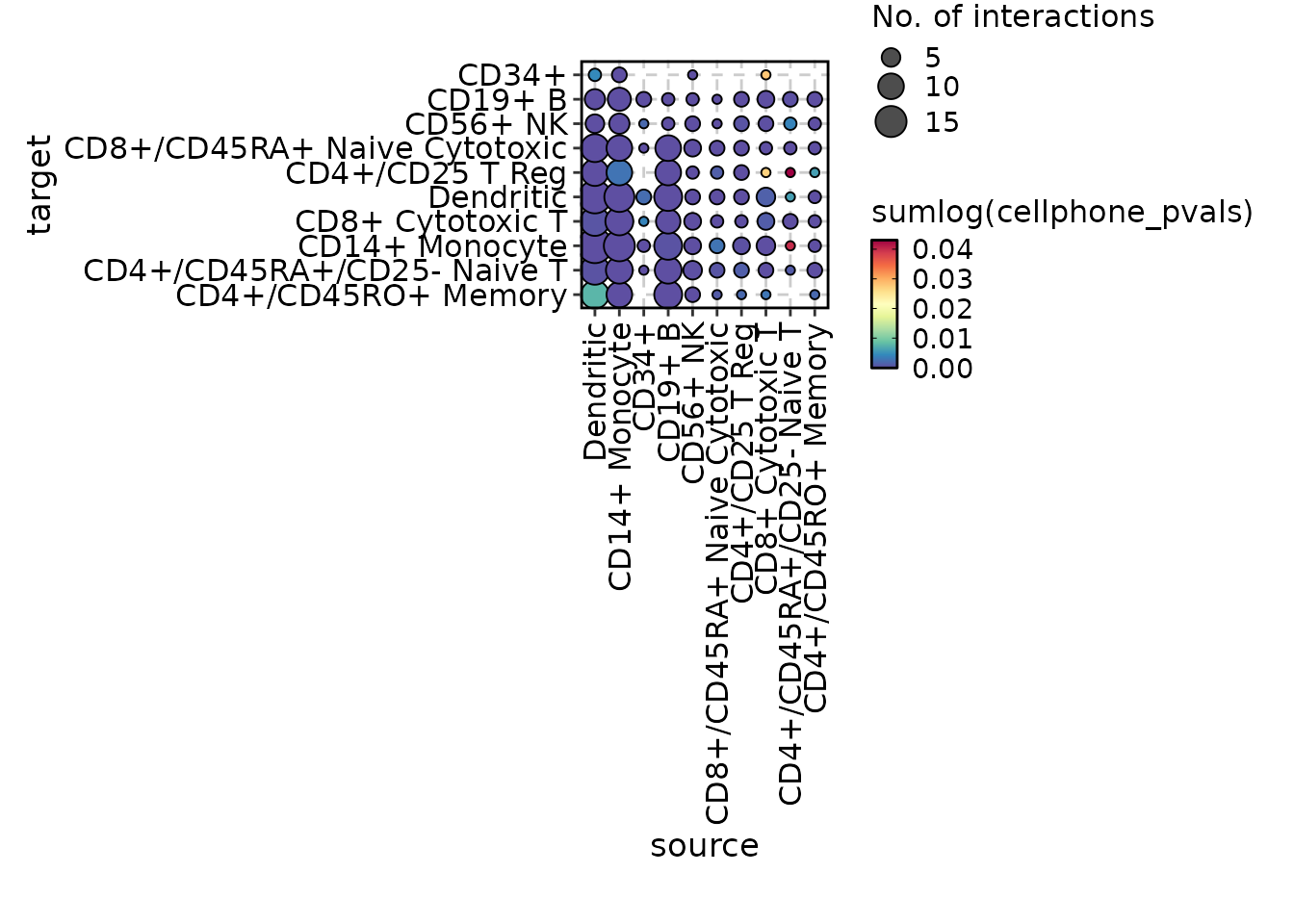
chat$ask("Generate a cell-cell communication plot for the cellphonedb_res data.")
#>
#> Tool identified:  CCCPlot
#>
#> Data object identified:  scplotter::cellphonedb_res
#> Warning in wrap$modify_fn(prompt_text, llm_provider): The 'skimr' package is
#> required to skim dataframes. Skim summary of dataframes currently not shown in
#> prompt
#> Code ran:
#> CCCPlot(data = cellphonedb_res, plot_type = "dot")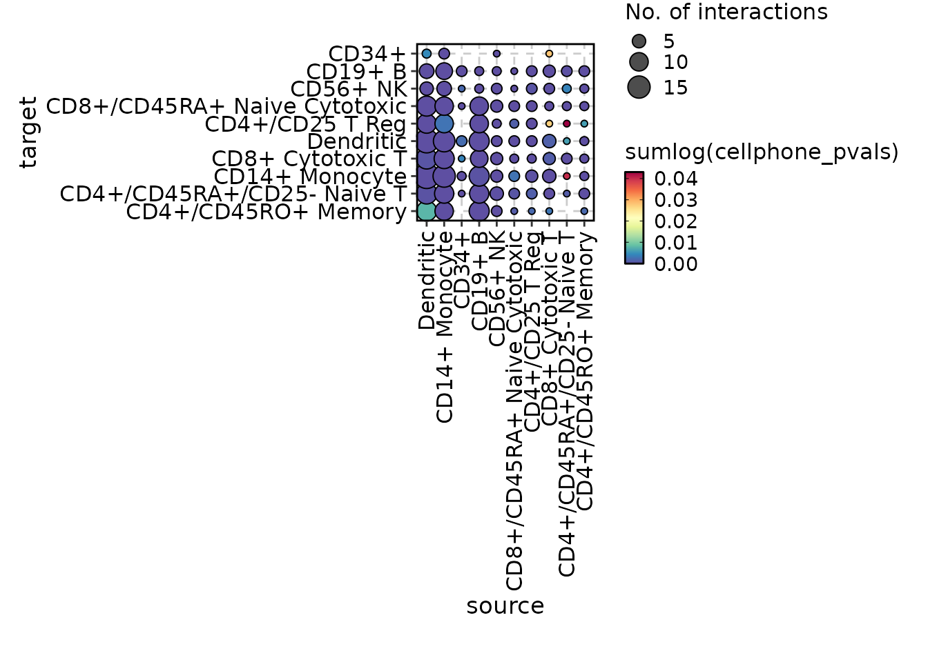
# Previous conversation is memorized
chat$ask("Do a heatmap instead")
#>
#> Tool identified:  CCCPlot
#>
#> Data object identified:  scplotter::cellphonedb_res
#> Warning in wrap$modify_fn(prompt_text, llm_provider): The 'skimr' package is
#> required to skim dataframes. Skim summary of dataframes currently not shown in
#> prompt
#> Code ran:
#> CCCPlot(data = cellphonedb_res, plot_type = "heatmap")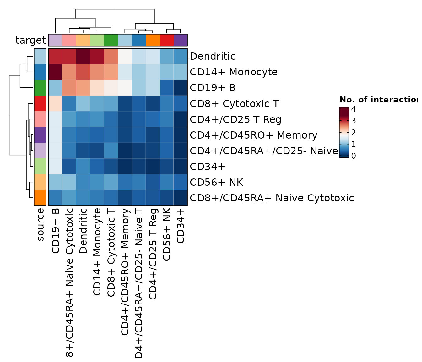
chat$ask("Add a proper title to the plot")
#>
#> Tool identified:  CCCPlot
#>
#> Data object identified:  scplotter::cellphonedb_res
#> Warning in wrap$modify_fn(prompt_text, llm_provider): The 'skimr' package is
#> required to skim dataframes. Skim summary of dataframes currently not shown in
#> prompt
#> Code ran:
#> CCCPlot(data = cellphonedb_res, plot_type = "heatmap", title = "Cell-Cell Communication Heatmap")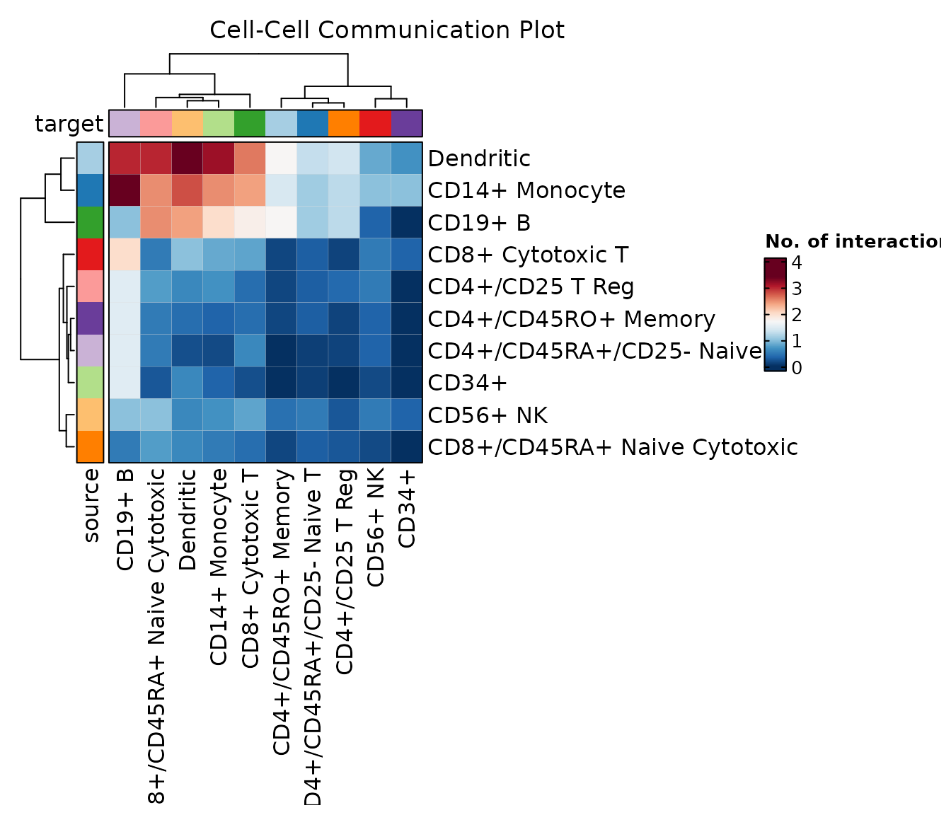
# To fetch the previous conversation
# Note that the response from the LLM is simplified in the history
chat$get_history()
#> [1] "User: Generate a cell-cell communication plot for the cellphonedb_res data."
#> [2] "Assistant: tool - CCCPlot; data - scplotter::cellphonedb_res; code - CCCPlot(data = cellphonedb_res, plot_type = \"dot\")"
#> [3] "User: Do a heatmap instead"
#> [4] "Assistant: tool - CCCPlot; data - scplotter::cellphonedb_res; code - CCCPlot(data = cellphonedb_res, plot_type = \"heatmap\")"
#> [5] "User: Add a proper title to the plot"
#> [6] "Assistant: tool - CCCPlot; data - scplotter::cellphonedb_res; code - CCCPlot(data = cellphonedb_res, plot_type = \"heatmap\", title = \"Cell-Cell Communication Heatmap\")"

# To clear the history
chat$clear_history()
Debug and improve the prompt
You can set verbose to TRUE for all
conversations when constructing the chat object. This will
print the prompt and the response from the LLM.
chat <- SCPlotterChat$new(
    provider = provider,
    verbose = TRUE
)
chat$ask("Generate a cell-cell communication plot for the cellphonedb_res data.")
#> --- Sending request to LLM provider (deepseek-v4-flash): ---
#> Objective: Select the most appropriate tool to handle the user's request while preserving conversational context. If the user refines or changes how the previous result should be visualized (e.g., asks for a different plot type), continue with the last plotting tool used unless they explicitly name a different tool.
#>
#> Decision Process:
#> - If the user explicitly names a tool, output that tool.
#> - Else, if the request appears to refine the previous output (e.g., "do X instead", "make it a heatmap/dot/bar/etc", "change to ...", "add ... to", "same plot but ..."), select the last tool mentioned in the chat history.
#> - Else, analyze the current user request; if there is a clear, unambiguous match to a single tool, select that tool.
#> - Else, use the last mentioned tool from the chat history.
#> - If no tool is found, respond with "None".
#>
#> Response Format: Provide only the name of the selected tool, or "None" if no tool applies.
#>
#> User Request:
#> Generate a cell-cell communication plot for the cellphonedb_res data.
#>
#> Available Tools:
#> - gt: Programmatic clone selection for TCR/BCR repertoire analysis
#>    Clone selectors provide a programmatic, expression-based system for filtering
#>    and selecting T cell and B cell clones from immune repertoire data. They are
#>    the foundation of clone-level analysis in    scplotter   , enabling flexible
#>    clone selection without manual specification of clone IDs.
#>
#>    Clone selectors operate on data frames containing clone abundance information
#>    (clone IDs paired with group-level counts or fractions). They evaluate
#>    selection criteria — such as abundance thresholds, group comparisons, or
#>    shared presence across conditions — and return either the selected clone IDs,
#>    a logical indicator vector, or a filtered data frame. The system is
#>    context-aware: it automatically detects whether it is being called from
#>    within a    dplyr    pipeline, a    scplotter    function, or standalone
#>    code, and adjusts its default behavior accordingly.
#>
#>    The following selector functions are available:
#>
#>        top()    — select the    n    largest clones by abundance
#>        sel()    — select clones matching a custom logical expression
#>        uniq()    — select clones unique to a specified group
#>        shared()    — select clones present in all specified groups
#>        gt()   ,    ge()   ,    lt()   ,    le()   ,    eq()   ,    ne()    — comparison-based selection
#>        and()   ,    or()    — combine multiple selector results
#>
#>
#> - CellDimPlot: Cell Dimension Reduction Plot
#>    Visualizes single-cell data in reduced dimension space (e.g., UMAP, t-SNE,
#>    PCA). This is the primary function for exploring cell clustering, cell
#>    identity, and spatial relationships in transcriptomics datasets. It creates
#>    scatter plots where each point represents a cell, positioned by its
#>    coordinates in the reduced dimension space and colored by metadata variables
#>    such as cell type, sample condition, or cluster assignment.
#>
#>    CellDimPlot    serves as a unified interface across multiple single-cell data
#>    containers:
#>
#>        Seurat objects    — Extracts embeddings from    Reductions()    and
#>    metadata from    @meta.data   . The default reduction is auto-detected
#>    via    default_dimreduc()   .
#>        Giotto objects    — Extracts spatial dimension reductions and cell
#>    metadata using    spat_unit    and    feat_type    to identify the correct
#>    spatial unit and feature type.
#>        h5ad files    (.h5ad or opened    H5File   ) — Reads from    obsm    for
#>    embeddings and    obs    for metadata. Reduction names are automatically
#>    prefixed with    "X_"    when needed (e.g.,    "umap"    →    "X_umap"   ).
#>
#>
#>    Beyond basic cluster visualization,    CellDimPlot    supports a rich set of
#>    visual overlays and analytical enhancements:
#>
#>        Cluster highlighting    — Emphasize cells matching a logical
#>    expression while dimming others (   highlight   ).
#>        Group labels    — Add text labels at group centroids (   label   ,
#>    label_insitu   ).
#>        Group marks    — Draw boundary shapes around groups: ellipse,
#>    rectangle, or circle (   add_mark   ,    mark_type   ).
#>        Density contours    — Overlay 2D density estimates (   add_density   ).
#>        Neighbor graphs    — Draw edges between neighboring cells from
#>    k-NN or shared-nearest-neighbor graphs (   graph   ).
#>        Lineage trajectories    — Overlay pseudotime lineage curves
#>    (   lineages   ).
#>        Velocity arrows    — Overlay RNA velocity vectors on the embedding
#>    (   velocity   ). For dedicated velocity visualization with grid or
#>    stream plots, see    CellVelocityPlot   .
#>        Statistical charts    — Embed small bar, ring, or line charts at
#>    group positions showing composition of a second variable (   stat_by   ,
#>    stat_plot_type   ).
#>        Hexagonal binning    — Replace scatter points with binned hexagons
#>    for large datasets (   hex   ).
#>        3D visualization    — Plot three dimensions by specifying
#>    dims = 1:3   .
#>        Rasterization    — Render points as a raster image for performance
#>    with large cell counts (   raster   ).
#>
#>
#> - ClonalVolumePlot: Clonal Volume Plot
#>    Visualizes the number (or fraction) of unique T-cell or B-cell clones across
#>    samples and metadata groups. Clonal volume — the count of distinct clonotypes
#>    detected in a sample — is a fundamental measure of immune repertoire diversity.
#>    Higher clonal volume indicates a more diverse repertoire, while lower volume
#>    may reflect clonal expansion in response to antigen stimulation.
#>
#>    ClonalVolumePlot    computes clonal counts via
#>    scRepertoire::clonalQuant()    and
#>    visualizes them as bar, box, or violin plots. It accepts both
#>    scRepertoire    combined TCR/BCR data and Seurat objects with clonal
#>    information integrated via    scRepertoire::combineExpression()   .
#>
#> - ClonalRarefactionPlot: Clonal Rarefaction Plot
#>    Visualizes clonal rarefaction curves — estimates of clone richness as a
#>    function of sampling depth. Rarefaction addresses a fundamental challenge
#>    in immune repertoire analysis: the number of clones observed depends on
#>    how many cells are sequenced. By repeatedly subsampling (bootstrapping)
#>    the data at varying depths, rarefaction curves reveal whether the
#>    repertoire has been sampled to saturation or whether additional
#>    sequencing would uncover many more clones.
#>
#>    ClonalRarefactionPlot    extracts clone count data from the repertoire,
#>    optionally groups it by metadata columns, and generates rarefaction
#>    curves via    plotthis::RarefactionPlot()   .
#>    When    split_by    is specified, separate plots are generated for each split
#>    group and combined into a multi-panel layout.
#>
#> - ClonalStatPlot: Visualize clone abundance, frequency, and dynamics across groups
#>    ClonalStatPlot provides a unified interface for visualizing the abundance, frequency,
#>    and dynamics of T cell and B cell clones across experimental groups. It is the most
#>    versatile clone visualization function in scplotter, offering multiple plot types
#>    for different analytical purposes.
#>
#>    The function operates on the output of    scRepertoire::combineTCR()   ,
#>    scRepertoire::combineBCR()   , or
#>    scRepertoire::combineExpression()   . Clones are
#>    identified by their CDR3 amino acid sequence, nucleotide sequence, V(D)J gene usage,
#>    or a combination thereof (via    clone_call   ). The function then computes clone-level
#>    statistics (size, fraction, or count of clones) within each group and renders them
#>    using one of ten supported plot types.
#>
#>    A defining feature of ClonalStatPlot is its flexible clone selection system. Clones
#>    can be specified directly by their IDs, or selected programmatically using expression
#>    selectors such as    top()   ,    sel()   ,    shared()   ,    uniq()   , and
#>    comparison operators (   gt()   ,    lt()   ,    eq()   , etc.). These selectors
#>    evaluate within the context of each faceting/splitting group, enabling per-group
#>    selection of the most expanded clones, clones shared between conditions, or clones
#>    meeting custom abundance thresholds. See the    Clone selection    section below
#>    and    CloneSelectors    for full details.
#>
#>    Clones can also be aggregated into named groups (by passing a named list to
#>    clones   ), where each group is defined by its own selection expression. In
#>    this mode, the visualization unit becomes the clone group rather than individual
#>    clones, enabling comparisons such as "hyper-expanded clones in condition A" vs.
#>    "hyper-expanded clones in condition B."
#>
#> - ClonalCompositionPlot: Clonal Composition Plot
#>    Visualizes the composition of the immune repertoire by categorizing clones
#>    into abundance groups (Rare, Small, Medium, Large, Hyperexpanded) and
#>    plotting their relative proportions across samples or metadata groups.
#>    This reveals the overall structure of the repertoire — whether it is
#>    dominated by a few large clones (clonal expansion) or composed of many
#>    small clones (high diversity).
#>
#>    ClonalCompositionPlot    supports three analysis methods:
#>
#>        Homeostasis    (   "homeostasis"   ,    "homeo"   ,    "rel"   ) —
#>    Clones are binned by their frequency (fraction of the total
#>    repertoire) into categories such as Rare, Small, Medium, Large,
#>    and Hyperexpanded. Uses
#>    scRepertoire::clonalHomeostasis()   .
#>        Top clones    (   "top"   ) — Clones are ranked and binned by
#>    their rank index (e.g., top 10, top 100, etc.). Uses
#>    scRepertoire::clonalProportion()   .
#>        Rare clones    (   "rare"   ) — Clones are binned by their
#>    absolute size (clone count). Uses clone size thresholds directly.
#>
#>
#> - EnrichmentPlot: Visualize gene set enrichment and over-representation analysis results
#>    Gene set enrichment analysis identifies biological pathways, gene ontologies,
#>    or functional categories that are statistically over-represented among a list
#>    of genes of interest (e.g., differentially expressed genes from a single-cell
#>    RNA-seq experiment). Rather than interpreting individual genes in isolation,
#>    enrichment analysis places gene-level results into a broader biological context,
#>    revealing which processes, functions, or diseases are perturbed.
#>
#>    EnrichmentPlot    generates publication-quality visualizations for enrichment
#>    results across eight distinct plot types, each suited to a different analytical
#>    perspective:
#>
#>        bar    — Horizontal bar chart of the top enriched terms, ordered by
#>    significance. Best for a quick overview or when showing a small number of terms.
#>        dot    — Dot plot where x-axis shows a continuous metric (default:
#>    GeneRatio   ), dot size reflects gene count, and dot color reflects
#>    significance. Ideal for comparing terms along two dimensions simultaneously.
#>        lollipop    — Lollipop chart combining dot and bar aesthetics.
#>    Similar to the dot plot but with stems emphasizing the ranking.
#>        comparison    — Side-by-side dot plot comparing enrichment across
#>    groups (e.g., cell types, conditions). Requires    group_by   .
#>        network    — Network visualization where nodes are enriched terms
#>    and edges represent overlapping gene sets. Reveals functional modules and
#>    redundant terms.
#>        enrichmap    — Enrichment map similar to the network plot but
#>    optimized for large term sets (default    top_term = 100   ). Nodes are
#>    terms and edges represent gene overlap.
#>        wordcloud    — Word cloud where term size reflects significance.
#>    Can display either enrichment terms (   word_type = "term"   ) or
#>    individual gene symbols (   word_type = "feature"   ).
#>        heatmap    — Heatmap of enrichment significance across groups
#>    (   group_by    is mapped to columns). Useful for comparing enrichment
#>    patterns across multiple conditions or cell types.
#>
#>
#>    The function auto-detects the input data format (   clusterProfiler    or
#>    enrichR   ) and delegates visualization to the appropriate    plotthis
#>    plotting function.
#>
#> - eq: Programmatic clone selection for TCR/BCR repertoire analysis
#>    Clone selectors provide a programmatic, expression-based system for filtering
#>    and selecting T cell and B cell clones from immune repertoire data. They are
#>    the foundation of clone-level analysis in    scplotter   , enabling flexible
#>    clone selection without manual specification of clone IDs.
#>
#>    Clone selectors operate on data frames containing clone abundance information
#>    (clone IDs paired with group-level counts or fractions). They evaluate
#>    selection criteria — such as abundance thresholds, group comparisons, or
#>    shared presence across conditions — and return either the selected clone IDs,
#>    a logical indicator vector, or a filtered data frame. The system is
#>    context-aware: it automatically detects whether it is being called from
#>    within a    dplyr    pipeline, a    scplotter    function, or standalone
#>    code, and adjusts its default behavior accordingly.
#>
#>    The following selector functions are available:
#>
#>        top()    — select the    n    largest clones by abundance
#>        sel()    — select clones matching a custom logical expression
#>        uniq()    — select clones unique to a specified group
#>        shared()    — select clones present in all specified groups
#>        gt()   ,    ge()   ,    lt()   ,    le()   ,    eq()   ,    ne()    — comparison-based selection
#>        and()   ,    or()    — combine multiple selector results
#>
#>
#> - CellVelocityPlot: Cell Velocity Plot
#>    Visualizes RNA velocity on a reduced-dimension embedding. RNA velocity
#>    infers the future transcriptional state of individual cells by modeling the
#>    ratio of unspliced (nascent) to spliced (mature) mRNA transcripts. On a
#>    dimension reduction plot, velocity is displayed as arrows (or grid/stream
#>    fields) showing the predicted direction and magnitude of transcriptional
#>    change for each cell — effectively revealing the "flow" of cells through
#>    differentiation, development, or other state transitions.
#>
#>    CellVelocityPlot    serves as a unified interface across multiple single-cell
#>    data containers:
#>
#>        Seurat objects    — Extracts embeddings from both the main
#>    reduction (   reduction   ) and the velocity reduction
#>    (   v_reduction   ) via    Embeddings()   ; metadata for grouping via
#>    @meta.data   .
#>        Giotto objects    — Extracts dimension reductions via
#>    getDimReduction()    using    spat_unit    and    feat_type    to identify
#>    the correct spatial unit and feature type.
#>        h5ad files    (.h5ad or opened    H5File   ) — Reads from    obsm    for
#>    both the main and velocity embeddings;    obs    for metadata. Reduction
#>    names are automatically prefixed with    "X_"    when needed.
#>
#>
#> - SpatFeaturePlot: Visualize feature expression on spatial coordinates
#>    Plot continuous feature values — gene expression, dimension reduction
#>    components, metadata columns, or any numeric variable — directly on
#>    spatial tissue coordinates.    SpatFeaturePlot()    is the spatial
#>    analogue of a feature plot over a UMAP/t-SNE embedding: it paints each
#>    spot, cell, or molecule with the expression level of one or more features,
#>    revealing the spatial organization of gene activity.
#>
#>    Multiple features are automatically faceted, making it easy to compare
#>    spatial expression patterns across a gene panel in a single plot. For
#>    categorical grouping (e.g., cluster identity on spatial coordinates), use
#>    SpatDimPlot    instead.
#>
#> - shared: Programmatic clone selection for TCR/BCR repertoire analysis
#>    Clone selectors provide a programmatic, expression-based system for filtering
#>    and selecting T cell and B cell clones from immune repertoire data. They are
#>    the foundation of clone-level analysis in    scplotter   , enabling flexible
#>    clone selection without manual specification of clone IDs.
#>
#>    Clone selectors operate on data frames containing clone abundance information
#>    (clone IDs paired with group-level counts or fractions). They evaluate
#>    selection criteria — such as abundance thresholds, group comparisons, or
#>    shared presence across conditions — and return either the selected clone IDs,
#>    a logical indicator vector, or a filtered data frame. The system is
#>    context-aware: it automatically detects whether it is being called from
#>    within a    dplyr    pipeline, a    scplotter    function, or standalone
#>    code, and adjusts its default behavior accordingly.
#>
#>    The following selector functions are available:
#>
#>        top()    — select the    n    largest clones by abundance
#>        sel()    — select clones matching a custom logical expression
#>        uniq()    — select clones unique to a specified group
#>        shared()    — select clones present in all specified groups
#>        gt()   ,    ge()   ,    lt()   ,    le()   ,    eq()   ,    ne()    — comparison-based selection
#>        and()   ,    or()    — combine multiple selector results
#>
#>
#> - CellStatPlot: Cell statistics plot
#>    Visualizes cell-level statistics — counts, fractions, and composition —
#>    across cell identities and metadata groupings. This is the primary function
#>    for exploring the distribution of cell types, clusters, and categorical
#>    metadata in single-cell transcriptomics datasets. It answers questions such
#>    as: "What proportion of each cell type is in each condition?", "How do
#>    cluster abundances change across samples?", and "What is the clonal
#>    composition within each cell type?"
#>
#>    CellStatPlot    serves as a unified interface across 15+ visualization
#>    types, all driven by a common data aggregation and fraction-calculation
#>    pipeline. It supports four single-cell data containers:
#>
#>        Seurat objects    — Extracts    @meta.data   ; uses    Idents()    as
#>    the default identity when    ident = NULL   .
#>        Giotto objects    — Extracts cell metadata via
#>    getCellMetadata()    using    spat_unit    and    feat_type   .
#>        h5ad files    (.h5ad or opened    H5File   ) — Reads from    obs
#>    via    h5group_to_dataframe()   .
#>        Data frames    — Internal method; all other methods ultimately
#>    delegate here after metadata extraction.
#>
#>
#> - ne: Programmatic clone selection for TCR/BCR repertoire analysis
#>    Clone selectors provide a programmatic, expression-based system for filtering
#>    and selecting T cell and B cell clones from immune repertoire data. They are
#>    the foundation of clone-level analysis in    scplotter   , enabling flexible
#>    clone selection without manual specification of clone IDs.
#>
#>    Clone selectors operate on data frames containing clone abundance information
#>    (clone IDs paired with group-level counts or fractions). They evaluate
#>    selection criteria — such as abundance thresholds, group comparisons, or
#>    shared presence across conditions — and return either the selected clone IDs,
#>    a logical indicator vector, or a filtered data frame. The system is
#>    context-aware: it automatically detects whether it is being called from
#>    within a    dplyr    pipeline, a    scplotter    function, or standalone
#>    code, and adjusts its default behavior accordingly.
#>
#>    The following selector functions are available:
#>
#>        top()    — select the    n    largest clones by abundance
#>        sel()    — select clones matching a custom logical expression
#>        uniq()    — select clones unique to a specified group
#>        shared()    — select clones present in all specified groups
#>        gt()   ,    ge()   ,    lt()   ,    le()   ,    eq()   ,    ne()    — comparison-based selection
#>        and()   ,    or()    — combine multiple selector results
#>
#>
#> - SpatDimPlot: Visualize categorical groups on spatial coordinates
#>    Plot categorical metadata — cluster identities, tissue regions, sample
#>    labels, or any discrete grouping variable — directly on spatial tissue
#>    coordinates.    SpatDimPlot()    is the spatial analogue of a UMAP/t-SNE
#>    plot colored by cluster: each spot, cell, or molecule is colored by its
#>    group membership, making it easy to assess the spatial organization of
#>    cell types, anatomical regions, or experimental conditions.
#>
#>    For continuous features (gene expression, dimension reduction scores),
#>    use    SpatFeaturePlot    instead.
#>
#> - GSEASummaryPlot: Objects exported from other packages
#>    These objects are imported from other packages. Follow the links
#>    below to see their documentation.
#>
#>
#>         plotthis   GSEAPlot()   ,    GSEASummaryPlot()
#>
#> - CCCPlot: Visualize Cell-Cell Communication (CCC) Interactions
#>    Cell-cell communication (CCC) is the process by which cells send and receive
#>    molecular signals — typically through ligand-receptor (LR) interactions — to
#>    coordinate tissue function. CCC analysis infers these interactions from
#>    single-cell transcriptomics data by identifying which ligand-receptor pairs
#>    are expressed between which cell types, often scoring each interaction by
#>    its magnitude (e.g., expression level, interaction score) and specificity
#>    (e.g., a p-value quantifying how cell-type-specific the interaction is).
#>
#>    CCCPlot    provides a unified interface to visualize CCC inference results
#>    (from tools like CellPhoneDB, LIANA, CellChat, NicheNet, etc.) across many
#>    plot types. It supports two fundamental modes:
#>
#>    Aggregation mode    (   method = "aggregation"   , the default): Ligand-receptor
#>    pairs are aggregated per source-target cell type pair. This shows    which
#>    cell types communicate    and how strongly. Supported plot types:    "network"   ,
#>    "chord"   /   "circos"   ,    "heatmap"   ,    "sankey"   /   "alluvial"   ,    "dot"   .
#>
#>    Interaction mode    (   method = "interaction"   ): Individual ligand-receptor
#>    pairs are plotted. This shows    which specific LR pairs    mediate the
#>    communication. Supported plot types:    "dot"   ,    "network"   ,    "heatmap"   ,
#>    "box"   ,    "violin"   ,    "ridge"   .
#>
#>    The    "linkedheatmap"    plot type is a special case: it does not use the
#>    method    parameter. It displays a side-by-side heatmap where the left side
#>    shows ligand expression across source cell types and the right side shows
#>    receptor expression across target cell types, with links between them
#>    representing the LR pairs. This plot type requires    ligand_means    and
#>    receptor_means    columns.
#>
#>    Under the hood,    CCCPlot    preprocesses the data (aggregating or
#>    reformatting as needed) and delegates rendering to the corresponding
#>    plotthis    package function. All styling and layout arguments accepted by
#>    those functions can be passed through    ...   .
#>
#> - ClonalResidencyPlot: Clonal Residency Plot
#>    Visualizes the sharing (residency) of T-cell or B-cell clones across
#>    different samples or metadata groups. Clonal residency analysis reveals
#>    how clonotypes are distributed — whether a clone is private to one
#>    condition or shared across multiple conditions — which is critical for
#>    understanding immune responses, tracking antigen-specific clones, and
#>    identifying public vs. private repertoires.
#>
#>    ClonalResidencyPlot    supports three visualization modes:
#>
#>        Scatter plot    — Compares clone sizes between two groups on
#>    log-transformed axes. Points are colored by clonal category:
#>    singletons (unique to one group), expanded clones, and dual
#>    clones (shared between groups). Correlation statistics are
#>    displayed in the subtitle.
#>        Venn diagram    — Shows the overlap of clone sets between up
#>    to 4 groups. When    with_class = TRUE   , labels include singlet
#>    counts.
#>        UpSet plot    — Shows intersection sizes for any number of
#>    groups. When    with_class = TRUE   , clone classes (singlet,
#>    expanded) are displayed as separate intersections.
#>
#>
#> - ClustreePlot: Visualize cluster stability across clustering resolutions
#>    A clustree plot visualizes how cells move between clusters when clustering is
#>    performed at different resolutions. Each resolution level is a column of nodes,
#>    and edges show the flow of cells between clusters at adjacent resolutions.
#>    This is an essential diagnostic for single-cell analysis, helping researchers
#>    choose an appropriate clustering resolution by revealing which clusters are
#>    stable (persistent across resolutions) and which are transient (appear only at
#>    specific resolutions).
#>
#>    This function is a wrapper around    plotthis::ClustreePlot()
#>    that automatically extracts the metadata from Seurat objects. For data frames,
#>    the data is passed directly to    plotthis   .
#>
#> - ClonalKmerPlot: Visualize CDR3 k-mer (motif) frequency
#>    Short amino acid motifs within CDR3 sequences — termed    k-mers    — can reveal
#>    shared binding specificities, common structural elements, and repertoire-level
#>    sequence features that are not apparent from full-length sequence analysis
#>    alone. Specific k-mers may be enriched in responses to particular antigens,
#>    represent public TCR/BCR motifs shared across individuals, or reflect
#>    convergent recombination events.
#>
#> - ClonalPositionalPlot: Visualize positional properties of CDR3 sequences
#>    The complementarity-determining region 3 (CDR3) is the most variable region of
#>    T cell and B cell receptors, and is the primary determinant of antigen
#>    specificity. Analyzing how amino acid composition, diversity, and
#>    physicochemical properties vary across CDR3 positions provides insight into
#>    repertoire structure, selection pressures, and the biophysical constraints
#>    that shape antigen recognition.
#>
#> - uniq: Programmatic clone selection for TCR/BCR repertoire analysis
#>    Clone selectors provide a programmatic, expression-based system for filtering
#>    and selecting T cell and B cell clones from immune repertoire data. They are
#>    the foundation of clone-level analysis in    scplotter   , enabling flexible
#>    clone selection without manual specification of clone IDs.
#>
#>    Clone selectors operate on data frames containing clone abundance information
#>    (clone IDs paired with group-level counts or fractions). They evaluate
#>    selection criteria — such as abundance thresholds, group comparisons, or
#>    shared presence across conditions — and return either the selected clone IDs,
#>    a logical indicator vector, or a filtered data frame. The system is
#>    context-aware: it automatically detects whether it is being called from
#>    within a    dplyr    pipeline, a    scplotter    function, or standalone
#>    code, and adjusts its default behavior accordingly.
#>
#>    The following selector functions are available:
#>
#>        top()    — select the    n    largest clones by abundance
#>        sel()    — select clones matching a custom logical expression
#>        uniq()    — select clones unique to a specified group
#>        shared()    — select clones present in all specified groups
#>        gt()   ,    ge()   ,    lt()   ,    le()   ,    eq()   ,    ne()    — comparison-based selection
#>        and()   ,    or()    — combine multiple selector results
#>
#>
#> - top: Programmatic clone selection for TCR/BCR repertoire analysis
#>    Clone selectors provide a programmatic, expression-based system for filtering
#>    and selecting T cell and B cell clones from immune repertoire data. They are
#>    the foundation of clone-level analysis in    scplotter   , enabling flexible
#>    clone selection without manual specification of clone IDs.
#>
#>    Clone selectors operate on data frames containing clone abundance information
#>    (clone IDs paired with group-level counts or fractions). They evaluate
#>    selection criteria — such as abundance thresholds, group comparisons, or
#>    shared presence across conditions — and return either the selected clone IDs,
#>    a logical indicator vector, or a filtered data frame. The system is
#>    context-aware: it automatically detects whether it is being called from
#>    within a    dplyr    pipeline, a    scplotter    function, or standalone
#>    code, and adjusts its default behavior accordingly.
#>
#>    The following selector functions are available:
#>
#>        top()    — select the    n    largest clones by abundance
#>        sel()    — select clones matching a custom logical expression
#>        uniq()    — select clones unique to a specified group
#>        shared()    — select clones present in all specified groups
#>        gt()   ,    ge()   ,    lt()   ,    le()   ,    eq()   ,    ne()    — comparison-based selection
#>        and()   ,    or()    — combine multiple selector results
#>
#>
#> - le: Programmatic clone selection for TCR/BCR repertoire analysis
#>    Clone selectors provide a programmatic, expression-based system for filtering
#>    and selecting T cell and B cell clones from immune repertoire data. They are
#>    the foundation of clone-level analysis in    scplotter   , enabling flexible
#>    clone selection without manual specification of clone IDs.
#>
#>    Clone selectors operate on data frames containing clone abundance information
#>    (clone IDs paired with group-level counts or fractions). They evaluate
#>    selection criteria — such as abundance thresholds, group comparisons, or
#>    shared presence across conditions — and return either the selected clone IDs,
#>    a logical indicator vector, or a filtered data frame. The system is
#>    context-aware: it automatically detects whether it is being called from
#>    within a    dplyr    pipeline, a    scplotter    function, or standalone
#>    code, and adjusts its default behavior accordingly.
#>
#>    The following selector functions are available:
#>
#>        top()    — select the    n    largest clones by abundance
#>        sel()    — select clones matching a custom logical expression
#>        uniq()    — select clones unique to a specified group
#>        shared()    — select clones present in all specified groups
#>        gt()   ,    ge()   ,    lt()   ,    le()   ,    eq()   ,    ne()    — comparison-based selection
#>        and()   ,    or()    — combine multiple selector results
#>
#>
#> - MarkersPlot: Visualize differential expression markers
#>    Visualize differential expression (DE) results — typically the output of
#>    Seurat::FindMarkers()    or
#>    Seurat::FindAllMarkers()    — across a
#>    variety of plot types. You can also compose the DE results from other
#>    tools into a data frame with the required columns and use this function to visualize them.
#>
#>    MarkersPlot()    bridges the gap between DE
#>    testing and visualization by providing a unified interface for both
#>    summary-level DE visualizations    (volcano, jitter, heatmap, and dot
#>    plots of fold changes and significance) and    expression-level
#>    visualizations    (violin, box, bar, ridge, heatmap, and dot plots of actual
#>    expression values from a Seurat object).
#>
#>    The function handles two broad categories of plots:
#>
#>        DE summary plots    (no    object    required): visualize the
#>    DE statistics themselves — log2 fold change, percentage difference,
#>    p-values, and adjusted p-values — across groups or comparisons.
#>
#>        "volcano"    /    "volcano_log2fc"    — Volcano plot with
#>    log2 fold change on the x-axis and    -log_{10}(p)    on the y-axis.
#>    Genes passing the    cutoff    are highlighted and top genes are
#>    labeled. Ideal for overview of effect size vs. significance.
#>        "volcano_pct"    — Volcano plot with percentage-point
#>    difference (   pct.1 - pct.2   ) on the x-axis. Useful when the
#>    biological question is about detection rate rather than expression
#>    magnitude.
#>        "jitter"    /    "jitter_log2fc"    — Jitter plot of log2
#>    fold changes across groups (defined by    each   ). Dot size
#>    encodes    -log_{10}(p)   . Reveals distribution of effect sizes
#>    per cluster or condition.
#>        "jitter_pct"    — Jitter plot of percentage-point
#>    differences across groups.
#>        "heatmap_log2fc"    — Heatmap of log2 fold changes (genes
#>    × groups). Cells can be marked for significance via    cutoff
#>    and    sig_mark   .
#>        "heatmap_pct"    — Heatmap of percentage-point differences
#>    (genes × groups). Same significance-marking support.
#>        "dot_log2fc"    — Dot plot of log2 fold changes (genes ×
#>    groups). Dot size encodes    -log_{10}(p)   .
#>        "dot_pct"    — Dot plot of percentage-point differences
#>    (genes × groups). Dot size encodes    -log_{10}(p)   .
#>
#>        Expression plots    (   object    required): visualize the
#>    actual expression values of the selected marker genes in the context of
#>    the original Seurat object. These are useful for validating DE results
#>    by inspecting the underlying expression distributions.
#>
#>        "heatmap"    — Expression heatmap of selected marker genes.
#>        "violin"    — Violin plots of expression per gene.
#>        "box"    — Box plots of expression per gene.
#>        "bar"    — Bar plots of mean expression per gene.
#>        "ridge"    — Ridge plots of expression distribution per gene.
#>        "dot"    — Dot plot of expression (fraction expressing ×
#>    mean expression) per gene.
#>
#>
#>
#> - ClonalOverlapPlot: Clonal Overlap Plot
#>    Visualizes the overlap (sharing) of T-cell or B-cell clonotypes between
#>    samples or metadata groups as a heatmap. Each cell in the heatmap
#>    quantifies the degree of clonal sharing between two groups, using one of
#>    several similarity or overlap metrics. This is a key analysis for
#>    identifying public clones shared across individuals, tracking
#>    antigen-specific clones across time points or tissues, and comparing
#>    repertoire similarity between conditions.
#>
#>    ClonalOverlapPlot    computes pairwise overlap via
#>    scRepertoire::clonalOverlap()
#>    and visualizes the resulting matrix as a labeled heatmap using
#>    plotthis::Heatmap()   .
#>
#> - ge: Programmatic clone selection for TCR/BCR repertoire analysis
#>    Clone selectors provide a programmatic, expression-based system for filtering
#>    and selecting T cell and B cell clones from immune repertoire data. They are
#>    the foundation of clone-level analysis in    scplotter   , enabling flexible
#>    clone selection without manual specification of clone IDs.
#>
#>    Clone selectors operate on data frames containing clone abundance information
#>    (clone IDs paired with group-level counts or fractions). They evaluate
#>    selection criteria — such as abundance thresholds, group comparisons, or
#>    shared presence across conditions — and return either the selected clone IDs,
#>    a logical indicator vector, or a filtered data frame. The system is
#>    context-aware: it automatically detects whether it is being called from
#>    within a    dplyr    pipeline, a    scplotter    function, or standalone
#>    code, and adjusts its default behavior accordingly.
#>
#>    The following selector functions are available:
#>
#>        top()    — select the    n    largest clones by abundance
#>        sel()    — select clones matching a custom logical expression
#>        uniq()    — select clones unique to a specified group
#>        shared()    — select clones present in all specified groups
#>        gt()   ,    ge()   ,    lt()   ,    le()   ,    eq()   ,    ne()    — comparison-based selection
#>        and()   ,    or()    — combine multiple selector results
#>
#>
#> - ClonalLengthPlot: Clonal CDR3 Length Plot
#>    Visualizes the distribution of CDR3 sequence lengths across the immune
#>    repertoire. CDR3 length is a key feature of T-cell and B-cell receptor
#>    diversity — different clones have different CDR3 lengths, and shifts in
#>    length distribution can indicate clonal selection, antigen-specific
#>    expansion, or repertoire bias.
#>
#>    ClonalLengthPlot    computes CDR3 length data via
#>    scRepertoire::clonalLength()    and
#>    visualizes the distribution as bar, box, violin, or density plots. Length
#>    is measured in amino acids (when    clone_call = "aa"   ) or nucleotides
#>    (when    clone_call = "nt"   ).
#>
#> - and: Programmatic clone selection for TCR/BCR repertoire analysis
#>    Clone selectors provide a programmatic, expression-based system for filtering
#>    and selecting T cell and B cell clones from immune repertoire data. They are
#>    the foundation of clone-level analysis in    scplotter   , enabling flexible
#>    clone selection without manual specification of clone IDs.
#>
#>    Clone selectors operate on data frames containing clone abundance information
#>    (clone IDs paired with group-level counts or fractions). They evaluate
#>    selection criteria — such as abundance thresholds, group comparisons, or
#>    shared presence across conditions — and return either the selected clone IDs,
#>    a logical indicator vector, or a filtered data frame. The system is
#>    context-aware: it automatically detects whether it is being called from
#>    within a    dplyr    pipeline, a    scplotter    function, or standalone
#>    code, and adjusts its default behavior accordingly.
#>
#>    The following selector functions are available:
#>
#>        top()    — select the    n    largest clones by abundance
#>        sel()    — select clones matching a custom logical expression
#>        uniq()    — select clones unique to a specified group
#>        shared()    — select clones present in all specified groups
#>        gt()   ,    ge()   ,    lt()   ,    le()   ,    eq()   ,    ne()    — comparison-based selection
#>        and()   ,    or()    — combine multiple selector results
#>
#>
#> - ClonalAbundancePlot: Clonal Abundance Plot
#>    Visualizes the distribution of clonal abundances — how many clones are
#>    present at each abundance level (frequency) in the repertoire. Clonal
#>    abundance distributions typically follow a power-law pattern: a small
#>    number of highly expanded clones and a large number of rare clones.
#>    This function helps characterize repertoire structure by showing whether
#>    the immune response is dominated by a few large clones (clonal expansion)
#>    or evenly distributed across many clones (high diversity).
#>
#>    ClonalAbundancePlot    computes clonal abundance data via
#>    scRepertoire::clonalAbundance()
#>    and visualizes it as trend lines, histograms, or density curves.
#>
#> - sel: Programmatic clone selection for TCR/BCR repertoire analysis
#>    Clone selectors provide a programmatic, expression-based system for filtering
#>    and selecting T cell and B cell clones from immune repertoire data. They are
#>    the foundation of clone-level analysis in    scplotter   , enabling flexible
#>    clone selection without manual specification of clone IDs.
#>
#>    Clone selectors operate on data frames containing clone abundance information
#>    (clone IDs paired with group-level counts or fractions). They evaluate
#>    selection criteria — such as abundance thresholds, group comparisons, or
#>    shared presence across conditions — and return either the selected clone IDs,
#>    a logical indicator vector, or a filtered data frame. The system is
#>    context-aware: it automatically detects whether it is being called from
#>    within a    dplyr    pipeline, a    scplotter    function, or standalone
#>    code, and adjusts its default behavior accordingly.
#>
#>    The following selector functions are available:
#>
#>        top()    — select the    n    largest clones by abundance
#>        sel()    — select clones matching a custom logical expression
#>        uniq()    — select clones unique to a specified group
#>        shared()    — select clones present in all specified groups
#>        gt()   ,    ge()   ,    lt()   ,    le()   ,    eq()   ,    ne()    — comparison-based selection
#>        and()   ,    or()    — combine multiple selector results
#>
#>
#> - ClonalDiversityPlot: Clonal Diversity Plot
#>    Visualizes clonal diversity metrics across samples or metadata groups.
#>    Clonal diversity quantifies the richness and evenness of the immune
#>    repertoire — how many distinct clonotypes are present and how evenly
#>    cells are distributed among them. High diversity indicates a broad,
#>    well-distributed repertoire; low diversity may indicate clonal expansion
#>    (oligoclonality) in response to antigen stimulation or disease.
#>
#>    ClonalDiversityPlot    computes diversity scores using a custom
#>    implementation that wraps several    scRepertoire    methods and adds
#>    three    scplotter   -specific metrics (Gini coefficient, D50, DXX).
#>    Results are visualized as bar, box, or violin plots.
#>
#> - FeatureStatPlot: Visualize feature expression and statistics across cell groups
#>    A central question in single-cell analysis is how features — genes, gene
#>    signatures, module scores, or other molecular measurements — vary across cell
#>    types, conditions, or experimental groups.    FeatureStatPlot    answers this
#>    question by providing eight complementary visualization types, each suited to
#>    a different analytical perspective:
#>
#>        violin    — Violin plot showing the full distribution of feature
#>    values per identity group. Best for comparing expression distributions
#>    and detecting bimodality or outliers.
#>        box    — Box plot summarizing feature values with quartiles and
#>    outliers. A compact alternative to the violin plot.
#>        bar    — Bar chart of aggregated feature values (default: mean)
#>    per group. Useful for summary-level comparisons with error bars.
#>        ridge    — Ridge (joy) plot showing density curves per group.
#>    Effective when comparing many groups or when distribution shape matters.
#>        dim    — Dimensionality reduction plot (UMAP, t-SNE, PCA) with
#>    cells colored by feature expression. Reveals spatial patterns of gene
#>    expression in the reduced space.
#>        cor    — Correlation plot between two features (scatter with
#>    fitted line and annotations) or among multiple features (pairs plot).
#>    Reveals co-expression relationships.
#>        heatmap    — Heatmap of feature expression across identity
#>    groups. Supports rich annotations (row/column metadata, bar charts,
#>    pie charts, violin plots) and flexible clustering. The go-to choice
#>    for visualizing many features across many groups.
#>        dot    — Dot plot (a shortcut for heatmap with
#>    cell_type = "dot"   ) where dot size reflects the fraction of
#>    expressing cells and dot color reflects mean expression. A compact,
#>    publication-ready format for marker gene visualization.
#>
#>
#>    The function is an S3 generic with methods for    Seurat    objects,
#>    Giotto    objects, AnnData (.h5ad) file paths, and    H5File    objects
#>    (via    hdf5r   ). Each method extracts the relevant expression matrix and
#>    metadata, then delegates to the internal    .feature_stat_plot()    which
#>    dispatches to the appropriate    plotthis    plotting function.
#>
#> - ClonalGeneUsagePlot: Visualize TCR/BCR gene segment usage
#>    Adaptive immune receptors (TCRs and BCRs) are assembled through V(D)J recombination,
#>    where variable (V), diversity (D), and joining (J) gene segments are randomly selected
#>    and rearranged. The frequency with which different gene segments are used — termed
#>    gene usage    — provides insight into immune repertoire composition, T/B cell
#>    development, and antigen-driven selection. Skewed gene usage can indicate clonal
#>    expansion, immune aging, or disease-associated repertoire bias.
#>
#> - lt: Programmatic clone selection for TCR/BCR repertoire analysis
#>    Clone selectors provide a programmatic, expression-based system for filtering
#>    and selecting T cell and B cell clones from immune repertoire data. They are
#>    the foundation of clone-level analysis in    scplotter   , enabling flexible
#>    clone selection without manual specification of clone IDs.
#>
#>    Clone selectors operate on data frames containing clone abundance information
#>    (clone IDs paired with group-level counts or fractions). They evaluate
#>    selection criteria — such as abundance thresholds, group comparisons, or
#>    shared presence across conditions — and return either the selected clone IDs,
#>    a logical indicator vector, or a filtered data frame. The system is
#>    context-aware: it automatically detects whether it is being called from
#>    within a    dplyr    pipeline, a    scplotter    function, or standalone
#>    code, and adjusts its default behavior accordingly.
#>
#>    The following selector functions are available:
#>
#>        top()    — select the    n    largest clones by abundance
#>        sel()    — select clones matching a custom logical expression
#>        uniq()    — select clones unique to a specified group
#>        shared()    — select clones present in all specified groups
#>        gt()   ,    ge()   ,    lt()   ,    le()   ,    eq()   ,    ne()    — comparison-based selection
#>        and()   ,    or()    — combine multiple selector results
#>
#>
#> - GSEAPlot: Objects exported from other packages
#>    These objects are imported from other packages. Follow the links
#>    below to see their documentation.
#>
#>
#>         plotthis   GSEAPlot()   ,    GSEASummaryPlot()
#>
#> - or: Programmatic clone selection for TCR/BCR repertoire analysis
#>    Clone selectors provide a programmatic, expression-based system for filtering
#>    and selecting T cell and B cell clones from immune repertoire data. They are
#>    the foundation of clone-level analysis in    scplotter   , enabling flexible
#>    clone selection without manual specification of clone IDs.
#>
#>    Clone selectors operate on data frames containing clone abundance information
#>    (clone IDs paired with group-level counts or fractions). They evaluate
#>    selection criteria — such as abundance thresholds, group comparisons, or
#>    shared presence across conditions — and return either the selected clone IDs,
#>    a logical indicator vector, or a filtered data frame. The system is
#>    context-aware: it automatically detects whether it is being called from
#>    within a    dplyr    pipeline, a    scplotter    function, or standalone
#>    code, and adjusts its default behavior accordingly.
#>
#>    The following selector functions are available:
#>
#>        top()    — select the    n    largest clones by abundance
#>        sel()    — select clones matching a custom logical expression
#>        uniq()    — select clones unique to a specified group
#>        shared()    — select clones present in all specified groups
#>        gt()   ,    ge()   ,    lt()   ,    le()   ,    eq()   ,    ne()    — comparison-based selection
#>        and()   ,    or()    — combine multiple selector results
#>
#>
#> - ListTools: List all available tools
#> List all available tools that can be used to handle the chat request.
#>
#> - ListData: List all available data objects
#> List all available data objects that can be used to handle the chat request.
#> --- Receiving response from LLM provider: ---
#> CCCPlot
#> Tool identified:  CCCPlot
#> --- Sending request to LLM provider (deepseek-v4-flash): ---
#> Objective: Identify the data object to be used.
#>
#> Decision Process:
#> - If the user explicitly names a data object, output that data object name. If the name does not match exactly the available ones, use the one that is mostly related.
#> - Else, if the request appears to refine the previous output (e.g., "do X instead", "make it a heatmap/dot/bar/etc", "change to ...", "add ... to", "same plot but ..."), select the last dataset name mentioned in the chat history.
#> - Else, analyze the current user request; if there is a clear, unambiguous match to a dataset, select that data object.
#> - Else, use the last mentioned data object from the chat history.
#> - If no data object is found, respond with "None".
#>
#> Response Format: Provide only the name of the selected data object, or "None" if no tool applies. The response should be unquoted.
#>
#> User Request:
#> Generate a cell-cell communication plot for the cellphonedb_res data.
#>
#> Available Data Objects:
#> - scplotter::cellphonedb_res: A toy example of CellPhoneDB output from LIANA
#> - scplotter::ifnb_sub: A subsetted version of 'ifnb' datasets
#> - scplotter::pancreas_sub: A subsetted version of mouse 'pancreas' datasets
#> - Seurat::cc.genes: Cell cycle genes
#> - Seurat::cc.genes.updated.2019: Cell cycle genes: 2019 update
#> - SeuratObject::pbmc_small: A small example version of the PBMC dataset
#> - scRepertoire::contig_list: A list of 8 single-cell T cell receptor sequences runs.
#> - scRepertoire::mini_contig_list: Processed subset of 'contig_list'
#> - scRepertoire::scRep_example: A Seurat object of 500 single T cells,
#> --- Receiving response from LLM provider: ---
#> scplotter::cellphonedb_res
#> Data object identified:  scplotter::cellphonedb_res
#> Warning in wrap$modify_fn(prompt_text, llm_provider): The 'skimr' package is
#> required to skim dataframes. Skim summary of dataframes currently not shown in
#> prompt
#> --- Sending request to LLM provider (deepseek-v4-flash): ---
#> Objective: Generate the R code to run the specified tool using the specified data object based on the user's request and the provided tool information.
#>
#> Decision Process:
#> - Analyze the user's request to understand what needs to be done with the specified tool and data object.
#> - When use the data object name, do not quote it.
#> - Refer to the provided tool information to understand the tool's usage, arguments, and examples.
#> - Consider any specific parameters or options mentioned in the user's request that need to be included in the tool call.
#> - If the user's request is ambiguous or lacks necessary details, refer to the chat history for additional context that may help clarify the intended use of the tool and data object.
#> - Construct the R code that correctly calls the tool with the specified data object, ensuring that all necessary arguments are included and correctly formatted.
#>
#> Response Format: Provide only the valid R code wrapped between "```r" and "```" to run the tool.
#>
#> Tool to be used: CCCPlot
#> Data object to be used: cellphonedb_res
#>
#> User Request:
#> Generate a cell-cell communication plot for the cellphonedb_res data.
#>
#> Tool Information:
#> - title
#> Visualize Cell-Cell Communication (CCC) Interactions
#> - description
#>
#> Cell-cell communication (CCC) is the process by which cells send and receive
#> molecular signals — typically through ligand-receptor (LR) interactions — to
#> coordinate tissue function. CCC analysis infers these interactions from
#> single-cell transcriptomics data by identifying which ligand-receptor pairs
#> are expressed between which cell types, often scoring each interaction by
#> its magnitude (e.g., expression level, interaction score) and specificity
#> (e.g., a p-value quantifying how cell-type-specific the interaction is).
#>
#> CCCPlot provides a unified interface to visualize CCC inference results
#> (from tools like CellPhoneDB, LIANA, CellChat, NicheNet, etc.) across many
#> plot types. It supports two fundamental modes:
#>
#> Aggregation mode ( method = "aggregation" , the default): Ligand-receptor
#> pairs are aggregated per source-target cell type pair. This shows which
#> cell types communicate and how strongly. Supported plot types: "network" ,
#> "chord" / "circos" , "heatmap" , "sankey" / "alluvial" , "dot" .
#>
#> Interaction mode ( method = "interaction" ): Individual ligand-receptor
#> pairs are plotted. This shows which specific LR pairs mediate the
#> communication. Supported plot types: "dot" , "network" , "heatmap" ,
#> "box" , "violin" , "ridge" .
#>
#> The "linkedheatmap" plot type is a special case: it does not use the
#> method parameter. It displays a side-by-side heatmap where the left side
#> shows ligand expression across source cell types and the right side shows
#> receptor expression across target cell types, with links between them
#> representing the LR pairs. This plot type requires ligand_means and
#> receptor_means columns.
#>
#> Under the hood, CCCPlot preprocesses the data (aggregating or
#> reformatting as needed) and delegates rendering to the corresponding
#> plotthis package function. All styling and layout arguments accepted by
#> those functions can be passed through ... .
#>
#> - usage
#>
#> CCCPlot(
#> data,
#> plot_type = c("dot", "network", "chord", "circos", "heatmap", "sankey", "alluvial",
#> "box", "violin", "ridge", "linkedheatmap"),
#> method = c("aggregation", "interaction"),
#> magnitude = waiver(),
#> specificity = waiver(),
#> ligand_expr = "ligand_means",
#> receptor_expr = "receptor_means",
#> magnitude_agg = length,
#> magnitude_name = "No. of interactions",
#> meta_specificity = "sumlog",
#> split_by = NULL,
#> x_text_angle = 90,
#> link_curvature = 0.2,
#> link_alpha = 0.6,
#> facet_by = NULL,
#> show_row_names = TRUE,
#> show_column_names = TRUE,
#> values_fill = 0,
#> right_row_dend_side = "right",
#> columns_split_by = NULL,
#> rows_split_by = NULL,
#> ...
#> )
#>
#> - arguments
#> - data: A data frame containing cell-cell communication inference
#> results. Must include the columns source, target, ligand, and
#> receptor (as character or factor). Typically also includes one or more
#> numeric columns for interaction magnitude and specificity. See the
#> Data format section above for details.
#> - plot_type: The type of visualization. Default is "dot".
#> Possible values:
#>
#> "network": Source and target cell types as nodes, interactions as
#> edges. Edge thickness encodes magnitude. Accepts link_curvature and
#> link_alpha styling. When method = "interaction", nodes are ligands
#> and receptors instead, colored by source-target pair.
#> "chord", "circos" (aliases): Chord diagram linking source and target
#> cell types. Only available with method = "aggregation".
#> "heatmap": Source cell types on rows, target cell types on columns,
#> magnitude encoded as fill color. When method = "interaction", rows are
#> individual LR pairs and columns are split by source.
#> "sankey", "alluvial" (aliases): Flow diagram from source to target
#> cell types. Only available with method = "aggregation".
#> "dot": Source vs target grid with dot size encoding magnitude and
#> (optionally) dot color encoding specificity. Available in both methods.
#> "box": Box plots of interaction strengths. Each panel is a source cell
#> type, x-axis is target cell type. Only available with
#> method = "interaction".
#> "violin": Violin plots of interaction strengths. Layout is the same as
#> "box". Only available with method = "interaction".
#> "ridge": Ridge (joy) plots of interaction strengths. Rows are target
#> cell types, faceted by source. Only available with
#> method = "interaction".
#> "linkedheatmap": Side-by-side heatmaps showing ligand expression
#> (left, by source cell types) and receptor expression (right, by target
#> cell types) with LR pair links between them. Requires ligand_expr and
#> receptor_expr columns. Does not use the method parameter.
#>
#> - method: How to represent the data. Default is "aggregation".
#>
#> "aggregation": Aggregate all LR pairs for each source-target cell type
#> combination. Plots show cell-type-level communication.
#> "interaction": Plot individual LR pairs. Plots show LR-pair-level
#> detail. A magnitude column is required.
#>
#> - magnitude: The name of the column to use as the communication
#> magnitude (e.g., "lrscore", "sca_weight"). When not specified
#> (default), the second-to-last column of data is used. The chosen column
#> must be numeric. For LIANA outputs, common magnitude columns include
#> "lrscore", "sca_weight", or "cellphonedb_pvalue" (after
#> transformation). See
#> https://liana-py.readthedocs.io/en/latest/notebooks/basic_usage.html#Tileplot
#> for available LIANA methods.
#> - specificity: The name of the column to use as the communication
#> specificity (e.g., a p-value such as "pvalue" or
#> "cellphonedb_pvalue"). When not specified (default), the last column of
#> data is used. The chosen column must be numeric. Set to NULL if your
#> method does not produce a specificity score.
#> - ligand_expr: The name of the column containing the mean (or otherwise
#> summarized) expression of the ligand. Default is "ligand_means". Only
#> used when plot_type = "linkedheatmap".
#> - receptor_expr: The name of the column containing the mean (or
#> otherwise summarized) expression of the receptor. Default is
#> "receptor_means". Only used when plot_type = "linkedheatmap".
#> - magnitude_agg: A function used to aggregate the magnitude values
#> across multiple LR pairs within each source-target group. Applied only in
#> method = "aggregation". Default is length(), which counts the number
#> of LR interactions. Common alternatives: mean(), sum(), median().
#> - magnitude_name: A label for the aggregated magnitude that appears in
#> plot legends and axis titles. Default is "No. of interactions". Adjust
#> this to match magnitude_agg (e.g., use "Mean score" when
#> magnitude_agg = mean).
#> - meta_specificity: The meta-analysis method used to combine multiple
#> specificity p-values within each source-target group into a single
#> group-level p-value. Applied only in method = "aggregation" when a
#> specificity column is available. Default is "sumlog" (Fisher's method).
#> Must be one of the methods provided by the metap package:
#>
#> "invchisq": Inverse chi-squared method
#> "invt": Inverse t method
#> "logitp": Logit method
#> "meanp": Mean p method
#> "meanz": Mean z method
#> "sumlog": Sum of logs (Fisher's) method (default)
#> "sump": Sum of p (Edgington's) method
#> "two2one": Convert two-sided p-values to one-sided
#> "votep": Vote counting method
#> "wilkinsonp": Wilkinson's method
#>
#> - split_by: An optional character vector of column names used to
#> produce separate sub-plots (one per unique combination of values). When
#> NULL (default), a single plot is produced. For example, split by
#> a condition column to compare communication patterns across experimental
#> groups side-by-side.
#> - x_text_angle: The angle (in degrees) for the x-axis tick labels.
#> Used when plot_type is "dot" (both methods), "box", or "violin".
#> Default is 90 (vertical labels).
#> - link_curvature: The curvature of the edges in the network plot.
#> 0 gives straight lines; positive values curve edges outward. Default is
#> 0.2. Only used when plot_type = "network".
#> - link_alpha: The transparency (alpha) of the edges in the network
#> plot. Values range from 0 (fully transparent) to 1 (fully opaque).
#> Default is 0.6. Only used when plot_type = "network".
#> Only used when plot_type is "network" or linkedheatmap".
#> - facet_by: Deprecated. Not supported — must be NULL (the default).
#> Use split_by to produce separate plots instead.
#> - show_row_names: Whether to display row names in heatmap plots.
#> Default is TRUE. Used when plot_type is "heatmap" or
#> "linkedheatmap".
#> - show_column_names: Whether to display column names in heatmap plots.
#> Default is TRUE. Used when plot_type is "heatmap" or
#> "linkedheatmap".
#> - values_fill: The fill value for missing (NA) cells in the heatmap
#> matrix (e.g., when a source-target pair has no LR interactions). Default
#> is 0. Used when plot_type is "heatmap" or "linkedheatmap".
#> - right_row_dend_side: The side on which to place the row dendrogram
#> in the right-hand heatmap of the linked heatmap plot. Must be "left" or
#> "right". Default is "right". Only used when
#> plot_type = "linkedheatmap".
#> - columns_split_by: An optional character vector of column names used to
#> split the columns of the heatmap into separate blocks. Only used when
#> plot_type is "heatmap" or "linkedheatmap".
#> When method = "interaction", source is automatically used as a column split.
#> - rows_split_by: An optional character vector of column names used to
#> split the rows of the heatmap into separate blocks. Only used when
#> plot_type is "heatmap" or "linkedheatmap".
#> - ...: Additional arguments forwarded to the underlying plotthis
#> plotting function. The target function depends on plot_type:
#>
#> "network" → plotthis::Network()
#>
#> [...] can be:
#> - links: A data frame containing the edge list. Must contain the
#> from and to columns specifying source and target node
#> identifiers. Additional columns can be referenced by other parameters
#> (e.g., link_weight_by, link_type_by,
#> link_color_by).
#> - nodes: An optional data frame of node metadata. When provided,
#> columns such as node_size_by, node_color_by,
#> node_shape_by, and node_fill_by can reference its
#> columns. When NULL, the node set is inferred from the unique
#> values in the from and to columns. If a single character
#> string starting with "@", the nodes data frame is extracted
#> from the corresponding attribute of links (e.g.
#> "@nodes" extracts attr(links, "nodes")).
#> - split_by_sep: The separator for multiple split_by columns. See split_by
#> - split_nodes: A logical value. When TRUE and
#> split_by is provided, the nodes data frame is split by
#> the same split_by column in addition to the links. Both data
#> frames must have a column with the same name as split_by.
#> Default FALSE.
#> - from: A character string specifying the column name in
#> links for the source node identifiers. Defaults to
#> "from", or the first column of links if that column
#> name does not exist. Multiple columns can be provided; they are
#> concatenated with from_sep.
#> - from_sep: A character string to join multiple from
#> columns. Default "_". Ignored when from is a single
#> column.
#> - to: A character string specifying the column name in
#> links for the target node identifiers. Defaults to
#> "to", or the second column of links if that column
#> name does not exist. Multiple columns can be provided; they are
#> concatenated with to_sep.
#> - to_sep: A character string to join multiple to columns.
#> Default "_". Ignored when to is a single column.
#> - node_by: A character string specifying the column name in
#> nodes for the node identifiers. These must match the values
#> in the from / to columns of links. Defaults to
#> "name", or the first column of nodes if that column
#> name does not exist. Multiple columns can be provided; they are
#> concatenated with node_by_sep.
#> - node_by_sep: A character string to join multiple
#> node_by columns. Default "_". Ignored when
#> node_by is a single column.
#> - link_weight_by: A numeric value or a character string. If
#> numeric, all edges receive that constant line width. If a column
#> name, the edge line width is mapped to that column. Default
#> 2.
#> - link_weight_name: A character string for the link weight legend
#> title. When NULL (default), the column name from
#> link_weight_by is used. Only relevant when
#> link_weight_by is a column name.
#> - link_type_by: A character string or a column name specifying
#> the edge linetype. Can be "solid", "dashed",
#> "dotted", etc. If a column name from links is
#> supplied, the linetype is mapped to that column (with a version
#> check for ggplot2 4.0.0, where mapping is unsupported and a
#> warning is issued). Default "solid".
#> - link_type_name: A character string for the link linetype legend
#> title. When NULL (default), the column name from
#> link_type_by is used. Only relevant when
#> link_type_by is a column name.
#> - node_size_by: A numeric value or a character string. If
#> numeric, all nodes receive that constant point size. If a column
#> name, the size is mapped to that column. Default 15.
#> - node_size_name: A character string for the node size legend
#> title. When NULL (default), the column name from
#> node_size_by is used. Only relevant when
#> node_size_by is a column name.
#> - node_color_by: A character string specifying the node colour.
#> If a colour name or hex code (e.g. "black"), all nodes
#> receive that constant colour. If a column name from nodes is
#> supplied, the colour is mapped to that column. Default
#> "black".
#> - node_color_name: A character string for the node colour legend
#> title. When NULL (default), the column name from
#> node_color_by is used. Only relevant when
#> node_color_by is a column name.
#> - node_shape_by: A numeric value or a character string. If
#> numeric, all nodes receive that constant shape (see
#> shape). If a column name, the shape is
#> mapped to that column (cast to factor). Default 21 (filled
#> circle with border).
#> - node_shape_name: A character string for the node shape legend
#> title. When NULL (default), the column name from
#> node_shape_by is used. Only relevant when
#> node_shape_by is a column name.
#> - node_fill_by: A character string specifying the node fill
#> colour. If a colour name or hex code (e.g. "grey20"), all
#> nodes receive that constant fill. If a column name from
#> nodes is supplied, the fill is mapped to that column.
#> Default "grey20".
#> - node_fill_name: A character string for the node fill legend
#> title. When NULL (default), the column name from
#> node_fill_by is used. Only relevant when
#> node_fill_by is a column name.
#> - node_alpha: A numeric value specifying the fill transparency
#> of the nodes. Only applies when node_shape_by is one of the
#> filled shapes (21--25). Default 0.95.
#> - node_stroke: A numeric value specifying the border stroke
#> width of the node points. Default 1.5.
#> - cluster_scale: A character string specifying which node
#> aesthetic is overridden by cluster membership. One of
#> "fill", "color", or "shape". The value is
#> matched via match.arg; default is "fill".
#> - node_size_range: A numeric vector of length 2 giving the
#> minimum and maximum node size (in ggplot2 point units) when
#> node_size_by is a column name. Default c(5, 20).
#> - link_weight_range: A numeric vector of length 2 giving the
#> minimum and maximum edge line width (in mm) when
#> link_weight_by is a column name. Default
#> c(0.5, 5).
#> - link_arrow_offset: A numeric value (in points) specifying the
#> offset distance for the arrow end cap from the target node.
#> Prevents arrow heads from overlapping the node points. Only
#> relevant when directed = TRUE. Default 20.
#> - link_color_by: A character string controlling how edge colour
#> is determined. Options:
#>
#> "from" (default) -- colour follows the source node's
#> fill or colour aesthetic.
#> "to" -- colour follows the target node's fill or
#> colour.
#> A column name from links -- colour is mapped
#> directly to that column.
#>
#> - link_color_name: A character string for the edge colour legend
#> title. Only used when link_color_by is a column name (not
#> "from" or "to"). When NULL (default), the
#> column name is used.
#> - palette: A character string specifying the palette to use.
#> A named list or vector can be used to specify the palettes for different split_by values.
#> - palcolor: A character string specifying the color to use in the palette.
#> A named list can be used to specify the colors for different split_by values.
#> If some values are missing, the values from the palette will be used (palcolor will be NULL for those values).
#> - palreverse: A logical value indicating whether to reverse the palette. Default is FALSE.
#> - link_palette: A character string specifying the palette for
#> edge colours when they are mapped. When link_color_by is
#> "from" or "to", defaults to the node
#> palette. Otherwise defaults to "Set1".
#> - link_palcolor: A character vector specifying custom colours
#> for the edge palette. When link_color_by is "from"
#> or "to", defaults to the node palcolor. Otherwise
#> defaults to NULL.
#> - directed: A logical value. When TRUE, edges are drawn
#> with arrow heads and an end-cap offset. Default TRUE.
#> - layout: A character string or an igraph_layout_spec
#> object specifying the node placement algorithm. Built-in shortcuts:
#> "circle" (circular layout), "tree" (hierarchical
#> tree), "grid" (grid layout). Any other string is prefixed
#> with "layout_with_" and called as an igraph function (e.g.
#> "fr" for Fruchterman--Reingold, "kk" for
#> Kamada--Kawai). Default "circle".
#> - cluster: A character string specifying the community detection
#> algorithm. One of "none", "fast_greedy",
#> "walktrap", "edge_betweenness", "infomap", or
#> a custom clustering function from igraph. When not "none",
#> cluster membership overrides the aesthetic selected by
#> cluster_scale. Default "none".
#> - add_mark: A logical value. When TRUE (and
#> cluster != "none"), an enclosure mark is drawn around each
#> cluster's nodes. Default FALSE.
#> - mark_expand: A unit object specifying the
#> extra space around points within a cluster mark. Default
#> unit(10, "mm").
#> - mark_type: A character string specifying the mark geometry.
#> One of "hull", "ellipse", "rect", or
#> "circle", corresponding to ggforce's geom_mark_hull,
#> geom_mark_ellipse, geom_mark_rect, and
#> geom_mark_circle. The value is matched via
#> match.arg; default is "hull".
#> - mark_alpha: A numeric value for the fill transparency of
#> cluster marks. Default 0.1.
#> - mark_linetype: A numeric or character value specifying the
#> border line type of the cluster marks. Default 1 (solid).
#> - add_label: A logical value. When TRUE (default), node
#> identifiers are drawn as repulsive text labels via
#> geom_text_repel.
#> - label_size: A numeric value for the font size of node labels.
#> Scaled by the theme base size. Default 3.
#> - label_fg: A character string specifying the text colour of
#> node labels. Default "white".
#> - label_bg: A character string specifying the background colour
#> of node labels. Default "black".
#> - label_bg_r: A numeric value specifying the background box
#> radius (as a fraction of label height). Passed to
#> geom_text_repel's bg.r argument.
#> Default 0.1.
#> - arrow: A arrow object for the link
#> arrow heads. Only used when directed = TRUE. Default is
#> arrow(type = "closed", length = unit(0.1, "inches")).
#> - title: A character string specifying the title of the plot.
#> A function can be used to generate the title based on the default title.
#> This is useful when split_by is used and the title needs to be dynamic.
#> - subtitle: A character string specifying the subtitle of the plot.
#> - xlab: A character string specifying the x-axis label.
#> - ylab: A character string specifying the y-axis label.
#> - aspect.ratio: A numeric value specifying the aspect ratio of the plot.
#> - theme: A character string or a theme class (i.e. ggplot2::theme_classic) specifying the theme to use.
#> Default is "theme_this".
#> - theme_args: A list of arguments to pass to the theme function.
#> - legend.position: A character string specifying the position of the legend.
#> if waiver(), for single groups, the legend will be "none", otherwise "right".
#> - legend.direction: A character string specifying the direction of the legend.
#> - seed: The random seed to use. Default is 8525.
#> - combine: Whether to combine the plots into one when facet is FALSE. Default is TRUE.
#> - nrow: A numeric value specifying the number of rows in the facet.
#> - ncol: A numeric value specifying the number of columns in the facet.
#> - byrow: A logical value indicating whether to fill the plots by row.
#> - axes: A string specifying how axes should be treated. Passed to patchwork::wrap_plots().
#> Only relevant when split_by is used and combine is TRUE.
#> Options are:
#>
#> 'keep' will retain all axes in individual plots.
#> 'collect' will remove duplicated axes when placed in the same run of rows or columns of the layout.
#> 'collect_x' and 'collect_y' will remove duplicated x-axes in the columns or duplicated y-axes in the rows respectively.
#>
#> - axis_titles: A string specifying how axis titltes should be treated. Passed to patchwork::wrap_plots().
#> Only relevant when split_by is used and combine is TRUE.
#> Options are:
#>
#> 'keep' will retain all axis titles in individual plots.
#> 'collect' will remove duplicated titles in one direction and merge titles in the opposite direction.
#> 'collect_x' and 'collect_y' control this for x-axis titles and y-axis titles respectively.
#>
#> - guides: A string specifying how guides should be treated in the layout. Passed to patchwork::wrap_plots().
#> Only relevant when split_by is used and combine is TRUE.
#> Options are:
#>
#> 'collect' will collect guides below to the given nesting level, removing duplicates.
#> 'keep' will stop collection at this level and let guides be placed alongside their plot.
#> 'auto' will allow guides to be collected if a upper level tries, but place them alongside the plot if not.
#>
#> - design: Specification of the location of areas in the layout, passed to patchwork::wrap_plots().
#> Only relevant when split_by is used and combine is TRUE. When specified, nrow, ncol, and byrow are ignored.
#> See patchwork::wrap_plots() for more details.
#> "chord" / "circos" → plotthis::ChordPlot()
#>
#> [...] can be:
#> - y: A character string specifying the column name of the data frame to plot for the y-axis.
#> - from: A character string (or vector) specifying the column name(s)
#> for the source nodes. Character/factor columns are expected. Multiple
#> columns are concatenated with from_sep.
#> - from_sep: A character string to join multiple from columns.
#> Default "_".
#> - to: A character string (or vector) specifying the column name(s)
#> for the target nodes. Character/factor columns are expected. Multiple
#> columns are concatenated with to_sep.
#> - to_sep: A character string to join multiple to columns.
#> Default "_".
#> - split_by_sep: A character string to separate concatenated
#> split_by columns. Default "_".
#> - flip: Logical; if TRUE, swap the source and target nodes,
#> reversing the link direction.
#> - links_color: A character string controlling which node's colour
#> each link ribbon takes: "from" (default) or "to".
#> - theme: A character string or a theme class (i.e. ggplot2::theme_classic) specifying the theme to use.
#> Default is "theme_this".
#> - theme_args: A list of arguments to pass to the theme function.
#> - palette: A character string specifying the palette to use.
#> A named list or vector can be used to specify the palettes for different split_by values.
#> - palcolor: A character string specifying the color to use in the palette.
#> A named list can be used to specify the colors for different split_by values.
#> If some values are missing, the values from the palette will be used (palcolor will be NULL for those values).
#> - palreverse: A logical value indicating whether to reverse the palette. Default is FALSE.
#> - alpha: A numeric value specifying the transparency of the plot.
#> - labels_rot: Logical; if TRUE, rotate sector labels by 90
#> degrees (clockwise). Default FALSE uses niceFacing for
#> automatic orientation.
#> - title: A character string specifying the title of the plot.
#> A function can be used to generate the title based on the default title.
#> This is useful when split_by is used and the title needs to be dynamic.
#> - subtitle: A character string specifying the subtitle of the plot.
#> - seed: A numeric seed for reproducibility.
#> - keep_na: A logical value or a character to replace the NA values in the data.
#> It can also take a named list to specify different behavior for different columns.
#> If TRUE or NA, NA values will be replaced with NA.
#> If FALSE, NA values will be removed from the data before plotting.
#> If a character string is provided, NA values will be replaced with the provided string.
#> If a named vector/list is provided, the names should be the column names to apply the behavior to,
#> and the values should be one of TRUE, FALSE, or a character string.
#> Without a named vector/list, the behavior applies to categorical/character columns used on the plot,
#> for example, the x, group_by, fill_by, etc.
#> - keep_empty: One of FALSE, TRUE and "level". It can also take a named list to specify
#> different behavior for different columns. Without a named list, the behavior applies to the
#> categorical/character columns used on the plot, for example, the x, group_by, fill_by, etc.
#>
#> FALSE (default): Drop empty factor levels from the data before plotting.
#> TRUE: Keep empty factor levels and show them as a separate category in the plot.
#> "level": Keep empty factor levels, but do not show them in the plot.
#> But they will be assigned colors from the palette to maintain consistency across multiple plots.
#> Alias: levels
#>
#> - combine: Logical; when TRUE (default), returns a combined
#> patchwork object. When FALSE, returns a named list of
#> individual wrapped elements.
#> - ncol, nrow: Integer number of columns / rows for the combined layout.
#> - byrow: Logical; fill the combined layout by row (default TRUE).
#> - axes, axis_titles: Character strings for axis handling in the
#> combined layout.
#> - guides: Character string for legend collection across panels.
#> - design: A custom layout design for the combined plot.
#> "heatmap" → plotthis::Heatmap()
#>
#> [...] can be:
#> - values_by: A character of column name in data that contains the values to be plotted.
#> This is required when in_form is "long". For other formats, the values are pivoted into a column named by values_by.
#> - name: A character string to name the heatmap (will be used to rename values_by).
#> - in_form: The format of the data. Can be one of "matrix", "long", "wide-rows", "wide-columns", or "auto".
#> Defaults to "auto".
#> - split_by_sep: A character string to concat multiple columns in split_by.
#> - rows_by: A vector of column names in data that contains the row information.
#> This is used to create the rows of the heatmap.
#> When in_form is "long" or "wide-columns", this is requied, and multiple columns can be specified,
#> which will be concatenated by rows_by_sep into a single column.
#> - rows_by_sep: A character string to concat multiple columns in rows_by.
#> - rows_split_by_sep: A character string to concat multiple columns in rows_split_by.
#> - columns_by: A vector of column names in data that contains the column information.
#> This is used to create the columns of the heatmap.
#> When in_form is "long" or "wide-rows", this is required, and multiple columns can be specified,
#> which will be concatenated by columns_by_sep into a single column.
#> - columns_by_sep: A character string to concat multiple columns in columns_by.
#> - columns_split_by_sep: A character string to concat multiple columns in columns_split_by.
#> - rows_data: A data frame containing additional data for rows, which can be used to add annotations to the heatmap.
#> It will be joined to the main data by rows_by and split_by if split_by exists in rows_data.
#> This is useful for adding additional information to the rows of the heatmap.
#> - columns_data: A data frame containing additional data for columns, which can be used to add annotations to the heatmap.
#> It will be joined to the main data by columns_by and split_by if split_by exists in columns_data.
#> This is useful for adding additional information to the columns of the heatmap.
#> - keep_na: A logical value or a character to replace the NA values in the data.
#> It can also take a named list to specify different behavior for different columns.
#> If TRUE or NA, NA values will be replaced with NA.
#> If FALSE, NA values will be removed from the data before plotting.
#> If a character string is provided, NA values will be replaced with the provided string.
#> If a named vector/list is provided, the names should be the column names to apply the behavior to,
#> and the values should be one of TRUE, FALSE, or a character string.
#> Without a named vector/list, the behavior applies to categorical/character columns used on the plot,
#> for example, the x, group_by, fill_by, etc.
#> - keep_empty: One of FALSE, TRUE and "level". It can also take a named list to specify
#> different behavior for different columns. Without a named list, the behavior applies to the
#> categorical/character columns used on the plot, for example, the x, group_by, fill_by, etc.
#>
#> FALSE (default): Drop empty factor levels from the data before plotting.
#> TRUE: Keep empty factor levels and show them as a separate category in the plot.
#> "level": Keep empty factor levels, but do not show them in the plot.
#> But they will be assigned colors from the palette to maintain consistency across multiple plots.
#> Alias: levels
#>
#> - rows_orderby: A expression (in character) to specify how to order rows. It will be evaluated in the context of the data frame used for rows (after grouping by rows_split_by and rows_by). The expression should return a vector of the same length as the number of rows in the data frame. The default is NULL, which means no specific ordering.
#> Can't be used with cluster_rows = TRUE.
#> This is applied before renaming rows_by to rows_name.
#> - columns_orderby: A expression (in character) to specify how to order columns. It will be evaluated in the context of the data frame used for columns (after grouping by columns
#> split_by and columns_by). The expression should return a vector of the same length as the number of rows in the data frame. The default is NULL, which means no specific ordering.
#> Can't be used with cluster_columns = TRUE.
#> This is applied before renaming columns_by to columns_name.
#> - columns_name: A character string to rename the column created by columns_by, which will be reflected in the name of the annotation or legend.
#> - columns_split_name: A character string to rename the column created by columns_split_by, which will be reflected in the name of the annotation or legend.
#> - rows_name: A character string to rename the column created by rows_by, which will be reflected in the name of the annotation or legend.
#> - rows_split_name: A character string to rename the column created by rows_split_by, which will be reflected in the name of the annotation or legend.
#> - palette: A character string naming a palette (see
#> show_palettes) or a character vector of colours for the
#> main heatmap colour scale. Default "RdBu".
#> - palcolor: A custom colour vector overriding palette.
#> - palreverse: A logical value indicating whether to reverse the palette. Default is FALSE.
#> - pie_size_name: Legend title for the pie size.
#> - pie_size: A numeric value or function returning the pie radius.
#> When a function, it receives the count of groups in the pie.
#> - pie_values: A function or string (convertible via
#> match.arg) to compute the value represented by
#> each pie slice. Default "length" counts observations per
#> group.
#> - pie_name: A character string to rename the column created by pie_group_by, which will be reflected in the name of the annotation or legend.
#> - pie_group_by: A character of column name in data that contains the group information for pie charts.
#> This is used to create pie charts in the heatmap when cell_type is "pie".
#> - pie_group_by_sep: A character string to concat multiple columns in pie_group_by.
#> - pie_palette, pie_palcolor: Palette and custom colours for pie slice
#> fill colours.
#> - bars_sample: Fraction of each cell's observations (0 < x <= 1;
#> 1 uses all data) or a whole count > 1 sampled per cell when
#> cell_type = "bars". Column widths are proportional to the
#> number of bars drawn per column, so a numeric count gives equal
#> column widths and a fraction gives widths proportional to the
#> column data sizes. Proportional widths are skipped when
#> columns_split_by is given, and column clustering is
#> disabled in proportional mode. Default 1 (all data).
#> - label: A function to compute text labels when
#> cell_type = "label" (or "label+mark"). Receives the
#> aggregated value for a cell and optionally row/column indices and
#> names. See below for the full dispatch contract.
#> - label_size: Default point size for label text (used as fallback
#> when the label function does not return a size field).
#> - label_color: Default colour for label text (fallback).
#> - label_name: Legend title for the label colour scale. The legend
#> is shown automatically when the label function returns a
#> legend field for at least one cell.
#> - mark: A function to compute mark symbols when
#> cell_type = "mark" (or "label+mark"). Same dispatch
#> contract as label.
#> - mark_color: Default mark colour (fallback).
#> - mark_size: Default mark stroke width (lwd) in pt (fallback).
#> - mark_name: Legend title for the mark colour scale.
#> - violin_fill: A character vector of colours to use as fill for
#> violin plots when cell_type = "violin". If NULL, the
#> annotation colour is used.
#> - boxplot_fill: A character vector of colours to use as fill for
#> boxplots when cell_type = "boxplot". If NULL, the
#> annotation colour is used.
#> - dot_size: Dot size when cell_type = "dot". Can be a
#> numeric value or a function.
#> - dot_size_name: Legend title for the dot size.
#> - legend_items: A named numeric vector specifying custom legend
#> entries for the main colour scale. Names become the displayed labels.
#> - legend_discrete: Logical; if TRUE, treat the main colour
#> scale as discrete.
#> - legend.position: A character string specifying the position of the legend.
#> if waiver(), for single groups, the legend will be "none", otherwise "right".
#> - legend.direction: A character string specifying the direction of the legend.
#> - lower_quantile, upper_quantile, lower_cutoff, upper_cutoff: Quantile or explicit cutoffs for clipping the colour scale. Applied
#> to aggregated values for tile / label cell types; applied
#> to raw values for bars / violin / boxplot types.
#> - add_bg: Logical; if TRUE, add a background fill behind
#> non-tile cell types. Not used for cell_type = "tile" or
#> "bars".
#> - bg_alpha: Numeric in [0, 1] for background transparency.
#> - add_reticle: Logical; if TRUE, draw a reticle (crosshair
#> pattern) over the heatmap.
#> - reticle_color: Colour for the reticle lines.
#> - cluster_columns: Logical; cluster the columns. If TRUE and
#> columns_split_by is provided, clustering is applied within each
#> split group.
#> - cluster_rows: Logical; cluster the rows. If TRUE and
#> rows_split_by is provided, clustering is applied within each
#> split group.
#> - border: A logical value indicating whether to draw borders around
#> the heatmap. If TRUE, slice borders are also drawn. Default
#> TRUE.
#> - title: The global (column) title of the heatmap.
#> - column_title: Character string/vector used as the column group
#> annotation title. A character vector consisting entirely of the display
#> modes "inplace" (per-slice split titles), "legend" (split
#> annotation with legend, no title), "simple" (split annotation,
#> no legend/title), "anno" (alias "annotation"; label block
#> annotation) and "none" (no title, annotation, or legend)
#> controls how the split titles are displayed. A literal title identical
#> to a mode keyword is interpreted as a mode.
#> - row_title: Character string/vector used as the row group
#> annotation title. See column_title for the display modes.
#> - na_col: Colour for NA cells. Default "grey85".
#> - row_names_side: Side for row names. Default "right".
#> - column_names_side: Side for column names. Default "bottom".
#> - row_annotation: A structured list specifying row annotations.
#> Same format as column_annotation. Sides default to
#> "left". Aliases: .row/.rows for
#> rows_by, .row.split/.rows.split for
#> rows_split_by.
#> - row_annotation_side: Deprecated: use
#> row_annotation with the side sub-key instead.
#> - row_annotation_palette: Deprecated: use
#> row_annotation with the palette sub-key instead.
#> - row_annotation_palcolor: Deprecated: use
#> row_annotation with the palcolor sub-key instead.
#> - row_annotation_type: Deprecated: use
#> row_annotation with the type sub-key instead.
#> - row_annotation_params: Deprecated: use
#> row_annotation with the params sub-key instead.
#> - row_annotation_agg: Deprecated: use
#> row_annotation with the agg sub-key instead.
#> - column_annotation: A structured list specifying column annotations.
#> Each entry is a named list with sub-keys:
#>
#> colColumn name in data supplying the annotation
#> values. If omitted, the entry name is used as the column name.
#> side"top" or "bottom".
#> palettePalette name (see show_palettes).
#> palcolorCustom colour vector overriding palette.
#> typeAnnotation type: "auto", "simple",
#> "pie", "ring", "bar", "violin",
#> "boxplot", "density", "label",
#> "rownames", "points", "lines".
#> For split annotations, "rownames" (row splits) /
#> "colnames" (column splits) is like "label" but labels
#> each split block with the concatenated row/column names;
#> "names" and "dimnames" are aliases.
#> params$sep (default " ") controls the separator and
#> params$wrap_by the number of names per line.
#> For name annotations (the built-in rows_by/columns_by
#> annotation), "rownames"/"colnames" renders the
#> row/column names as text labels (this is what
#> show_row_names = "anno" uses).
#> paramsA list of additional parameters passed to the
#> annotation constructor. FALSE disables the annotation.
#> $show_legend controls legend visibility. See
#> HeatmapAnnotation.
#> aggA function to aggregate values for the annotation.
#> nameDisplay name for the annotation, shown next to the
#> annotation bar and used as the legend title. FALSE hides the
#> displayed name. Defaults to the annotation key (column name).
#>
#> Shortcuts:
#>
#> column_annotation = list(Score = "score") is short for
#> list(Score = list(col = "score")).
#> column_annotation = TRUE enables annotations with
#> defaults. FALSE disables all column annotations.
#>
#> Special keys:
#>
#> .default — default values inherited by all entries.
#> params is merged recursively; other keys are inherited
#> only when the entry does not already specify them.
#> .col / .cols / .column / .columns —
#> alias for columns_by (the built-in name annotation).
#> .col.split / .cols.split / .column.split /
#> .columns.split — alias for columns_split_by
#> (the built-in split annotation).
#> .row / .rows — alias for rows_by.
#> .row.split / .rows.split — alias for
#> rows_split_by.
#>
#> - column_annotation_side: Deprecated: use
#> column_annotation with the side sub-key instead.
#> - column_annotation_palette: Deprecated: use
#> column_annotation with the palette sub-key instead.
#> - column_annotation_palcolor: Deprecated: use
#> column_annotation with the palcolor sub-key instead.
#> - column_annotation_type: Deprecated: use
#> column_annotation with the type sub-key instead.
#> - column_annotation_params: Deprecated: use
#> column_annotation with the params sub-key instead.
#> - column_annotation_agg: Deprecated: use
#> column_annotation with the agg sub-key instead.
#> - flip: Logical; if TRUE, swap rows and columns
#> transparently. The caller does not need to swap row- and
#> column-related arguments manually.
#> - alpha: Alpha transparency for heatmap cells in [0, 1].
#> - seed: The random seed to use. Default is 8525.
#> - padding: Padding around the heatmap in CSS order (top, right,
#> bottom, left). Supports 1–4 values. Default 15 (mm). Note that
#> this is different from ComplexHeatmap::draw()'s padding
#> argument which uses bottom-left-top-right order.
#> - base_size: A positive numeric scalar used as a scaling factor for
#> the overall heatmap size. Default 1 (no scaling). Values > 1 enlarge
#> all cell dimensions proportionally.
#> - aspect.ratio: Height-to-width ratio of a single heatmap cell.
#> When NULL (default), sensible per-cell_type defaults are
#> used: 1 for tile/label/dot, 0.5 for bars,
#> and 2 for violin/boxplot/pie. The ratio is
#> constrained by the overall plot dimensions.
#> - draw_opts: A named list of additional arguments passed to
#> draw,HeatmapList-method. Internally
#> managed arguments take precedence.
#> - layer_fun_callback: A function to add custom graphical layers on
#> top of each heatmap cell. Receives j, i, x,
#> y, w, h, fill, sr, sc.
#> See Heatmap for details.
#> - cell_type: The type of cell to render. One of "tile"
#> (default), "bars", "label", "mark",
#> "label+mark" (or "mark+label"), "dot",
#> "violin", "boxplot", "pie". See the
#> Cell types section for details.
#> - cell_agg: A function to aggregate values within each cell when
#> cell_type = "tile" or "label". Default is
#> mean.
#> - combine: Whether to combine the plots into one when facet is FALSE. Default is TRUE.
#> - nrow: A numeric value specifying the number of rows in the facet.
#> - ncol: A numeric value specifying the number of columns in the facet.
#> - byrow: A logical value indicating whether to fill the plots by row.
#> - axes: A string specifying how axes should be treated. Passed to patchwork::wrap_plots().
#> Only relevant when split_by is used and combine is TRUE.
#> Options are:
#>
#> 'keep' will retain all axes in individual plots.
#> 'collect' will remove duplicated axes when placed in the same run of rows or columns of the layout.
#> 'collect_x' and 'collect_y' will remove duplicated x-axes in the columns or duplicated y-axes in the rows respectively.
#>
#> - axis_titles: A string specifying how axis titltes should be treated. Passed to patchwork::wrap_plots().
#> Only relevant when split_by is used and combine is TRUE.
#> Options are:
#>
#> 'keep' will retain all axis titles in individual plots.
#> 'collect' will remove duplicated titles in one direction and merge titles in the opposite direction.
#> 'collect_x' and 'collect_y' control this for x-axis titles and y-axis titles respectively.
#>
#> - guides: A string specifying how guides should be treated in the layout. Passed to patchwork::wrap_plots().
#> Only relevant when split_by is used and combine is TRUE.
#> Options are:
#>
#> 'collect' will collect guides below to the given nesting level, removing duplicates.
#> 'keep' will stop collection at this level and let guides be placed alongside their plot.
#> 'auto' will allow guides to be collected if a upper level tries, but place them alongside the plot if not.
#>
#> - design: Specification of the location of areas in the layout, passed to patchwork::wrap_plots().
#> Only relevant when split_by is used and combine is TRUE. When specified, nrow, ncol, and byrow are ignored.
#> See patchwork::wrap_plots() for more details.
#> "sankey" / "alluvial" → plotthis::SankeyPlot()
#>
#> [...] can be:
#> - in_form: A character string specifying the input data format.
#> One of "auto" (default), "long", "lodes",
#> "wide", "alluvia", or "counts".
#> "long" is an alias for "lodes"; "wide" is an alias for
#> "alluvia". See the data parameter of SankeyPlot
#> for format descriptions.
#> - x: A character string specifying the column name of the data frame to plot for the x-axis.
#> - x_sep: A character string to join multiple x columns when
#> in_form is "lodes" or auto-determined as lodes.
#> Default "_".
#> - y: A character string specifying the column name of the data frame to plot for the y-axis.
#> - stratum: A character string specifying the column that defines the
#> node categories at each x-axis position. Each unique value becomes a
#> stratum (node block) at each x position. When NULL, defaults to
#> links_fill_by. Multiple columns are concatenated with
#> stratum_sep. Ignored in "alluvia" format.
#> - stratum_sep: A character string to join multiple stratum
#> columns. Default "_".
#> - alluvium: A character string specifying the column that identifies
#> individual flows (alluvia) across x-axis positions. Each unique value
#> represents a single observational unit tracked across positions. When
#> NULL in "counts" format, an auto-generated identifier is
#> created. Multiple columns are concatenated with alluvium_sep.
#> Ignored in "alluvia" format.
#> - alluvium_sep: A character string to join multiple alluvium
#> columns. Default "_".
#> - split_by_sep: The separator for multiple split_by columns. See split_by
#> - keep_empty: One of FALSE, TRUE and "level". It can also take a named list to specify
#> different behavior for different columns. Without a named list, the behavior applies to the
#> categorical/character columns used on the plot, for example, the x, group_by, fill_by, etc.
#>
#> FALSE (default): Drop empty factor levels from the data before plotting.
#> TRUE: Keep empty factor levels and show them as a separate category in the plot.
#> "level": Keep empty factor levels, but do not show them in the plot.
#> But they will be assigned colors from the palette to maintain consistency across multiple plots.
#> Alias: levels
#>
#> - flow: A logical value. When FALSE (default),
#> geom_alluvium() is used for the links. When
#> TRUE, geom_flow() is used instead, which
#> draws the flows with a directional gradient between x positions.
#> - expand: The values to expand the x and y axes. It is like CSS padding.
#> When a single value is provided, it is used for both axes on both sides.
#> When two values are provided, the first value is used for the top/bottom side and the second value is used for the left/right side.
#> When three values are provided, the first value is used for the top side, the second value is used for the left/right side, and the third value is used for the bottom side.
#> When four values are provided, the values are used for the top, right, bottom, and left sides, respectively.
#> You can also use a named vector to specify the values for each side.
#> When the axis is discrete, the values will be applied as 'add' to the 'expansion' function.
#> When the axis is continuous, the values will be applied as 'mult' to the 'expansion' function.
#> See also https://ggplot2.tidyverse.org/reference/expansion.html
#> - nodes_legend: Controls how the node legend is displayed. One of:
#>
#> "auto" (default)Automatically determined:
#> if nodes_label = TRUE, or if stratum is identical to
#> links_fill_by with matching colours, the legend is hidden.
#> Otherwise, overlapping stratum values across x positions are checked:
#> any overlap produces a merged legend; no overlap produces separate
#> legends per x position.
#> "merge"A single merged legend for all nodes.
#> "separate"One legend per x-axis position, generated via
#> separate scale_fill_manual() layers.
#> "none"No node legend is shown.
#>
#> - nodes_color: A character string specifying the border colour of the
#> node (stratum) rectangles. Use the special value ".fill" to match
#> the border colour to the node fill colour. Default "grey30".
#> - links_fill_by: A character string specifying the column that
#> determines the fill colour of the links (alluvia / flows). When
#> NULL in "lodes" format, defaults to alluvium. In
#> "counts" format with the "." prefix, this parameter is
#> required. Multiple columns are concatenated with
#> links_fill_by_sep.
#> - links_fill_by_sep: A character string to join multiple
#> links_fill_by columns. Default "_".
#> - links_name: A character string for the legend title of the link fill
#> scale. When NULL (default), the links_fill_by column name
#> is used.
#> - links_color: A character string specifying the border colour of the
#> links (alluvia / flows). Use the special value ".fill" to match
#> the link border colour to the link fill colour. Default "gray80".
#> - nodes_palette: A character string specifying the colour palette for
#> the node (stratum) fill. Passed to palette_this().
#> Default "Paired".
#> - nodes_palcolor: A character vector of custom colours for the node
#> fill, used as palcolor in palette_this(). When
#> NULL (default), the palette colours are used directly.
#> - nodes_alpha: A numeric value in [0, 1] controlling the
#> transparency of the node (stratum) fill. Default 1.
#> - nodes_label: A logical value. When TRUE, stratum labels are
#> drawn inside each node using geom_label() with
#> StatStratum. Default FALSE.
#> - nodes_label_miny: A numeric value specifying the minimum y
#> (frequency) threshold for displaying node labels. Nodes with y-values
#> below this threshold are not labelled. Default 0.
#> - nodes_width: A numeric value (typically 0–1) specifying the width of
#> the node (stratum) rectangles as a fraction of the x-axis spacing.
#> Default 0.25.
#> - links_palette: A character string specifying the colour palette for
#> the link fill. Passed to palette_this().
#> Default "Paired".
#> - links_palcolor: A character vector of custom colours for the link
#> fill, used as palcolor in palette_this(). When
#> NULL (default), the palette colours are used directly.
#> - palreverse: A logical value indicating whether to reverse the palette. Default is FALSE.
#> - links_alpha: A numeric value in [0, 1] controlling the
#> transparency of the link fill. Default 0.6.
#> - legend.box: A character string specifying the arrangement of legend
#> boxes, either "vertical" (default) or "horizontal".
#> - aspect.ratio: A numeric value specifying the aspect ratio of the plot.
#> - legend.position: A character string specifying the position of the legend.
#> if waiver(), for single groups, the legend will be "none", otherwise "right".
#> - legend.direction: A character string specifying the direction of the legend.
#> - flip: A logical value. When TRUE,
#> coord_flip() is applied to swap the x and y axes.
#> Default FALSE.
#> - theme: A character string or a theme class (i.e. ggplot2::theme_classic) specifying the theme to use.
#> Default is "theme_this".
#> - theme_args: A list of arguments to pass to the theme function.
#> - title: A character string specifying the title of the plot.
#> A function can be used to generate the title based on the default title.
#> This is useful when split_by is used and the title needs to be dynamic.
#> - subtitle: A character string specifying the subtitle of the plot.
#> - xlab: A character string specifying the x-axis label.
#> - ylab: A character string specifying the y-axis label.
#> - facet_scales: Whether to scale the axes of facets. Default is "fixed"
#> Other options are "free", "free_x", "free_y". See ggplot2::facet_wrap
#> - facet_ncol: A numeric value specifying the number of columns in the facet.
#> When facet_by is a single column and facet_wrap is used.
#> - facet_nrow: A numeric value specifying the number of rows in the facet.
#> When facet_by is a single column and facet_wrap is used.
#> - facet_byrow: A logical value indicating whether to fill the plots by row. Default is TRUE.
#> - seed: The random seed to use. Default is 8525.
#> - combine: Whether to combine the plots into one when facet is FALSE. Default is TRUE.
#> - nrow: A numeric value specifying the number of rows in the facet.
#> - ncol: A numeric value specifying the number of columns in the facet.
#> - byrow: A logical value indicating whether to fill the plots by row.
#> - axes: A string specifying how axes should be treated. Passed to patchwork::wrap_plots().
#> Only relevant when split_by is used and combine is TRUE.
#> Options are:
#>
#> 'keep' will retain all axes in individual plots.
#> 'collect' will remove duplicated axes when placed in the same run of rows or columns of the layout.
#> 'collect_x' and 'collect_y' will remove duplicated x-axes in the columns or duplicated y-axes in the rows respectively.
#>
#> - axis_titles: A string specifying how axis titltes should be treated. Passed to patchwork::wrap_plots().
#> Only relevant when split_by is used and combine is TRUE.
#> Options are:
#>
#> 'keep' will retain all axis titles in individual plots.
#> 'collect' will remove duplicated titles in one direction and merge titles in the opposite direction.
#> 'collect_x' and 'collect_y' control this for x-axis titles and y-axis titles respectively.
#>
#> - guides: A string specifying how guides should be treated in the layout. Passed to patchwork::wrap_plots().
#> Only relevant when split_by is used and combine is TRUE.
#> Options are:
#>
#> 'collect' will collect guides below to the given nesting level, removing duplicates.
#> 'keep' will stop collection at this level and let guides be placed alongside their plot.
#> 'auto' will allow guides to be collected if a upper level tries, but place them alongside the plot if not.
#>
#> - design: Specification of the location of areas in the layout, passed to patchwork::wrap_plots().
#> Only relevant when split_by is used and combine is TRUE. When specified, nrow, ncol, and byrow are ignored.
#> See patchwork::wrap_plots() for more details.
#> "dot" → plotthis::DotPlot()
#>
#> [...] can be:
#> - x: A character string naming the column for the x-axis. Must be a
#> numeric column (bars extend from 0 to the data value).
#> - y: A character string naming the column for the y-axis. Must be a
#> factor or character column (each level gets a lollipop bar).
#> - x_sep: A character string used to join multiple x column values
#> into a single factor level. Only used when x is non-numeric and multiple
#> columns are provided. Default: "_".
#> - y_sep: A character string used to join multiple y column values
#> into a single factor level. Only used when y is non-numeric and multiple
#> columns are provided. Default: "_".
#> - flip: A logical value. If TRUE, the x and y axes are swapped via
#> coord_flip(). Dimension calculation accounts for the flip.
#> Default: FALSE.
#> - split_by_sep: A character string used to concatenate multiple
#> split_by column values. Default: "_".
#> - size_name: A character string for the size legend title. When
#> NULL (the default), the size_by column name is used.
#> - fill_name: A character string for the fill colour-bar legend title.
#> When NULL (the default), the fill_by column name is used.
#> - fill_cutoff_name: A character string for the fill cutoff legend title
#> (shown when fill_cutoff is active). Defaults to
#> "<fill_by> <fill_cutoff>", e.g. "mpg < 18".
#> - add_bg: A logical value. If TRUE, alternating background
#> stripes are drawn behind the points via bg_layer(). The
#> striped axis is determined by bg_direction. Requires the striped
#> axis to be non-numeric. Default: FALSE.
#> - bg_palette: A character string specifying the palette for the
#> background stripe colours. Passed to bg_layer().
#> Default: "stripe".
#> - bg_palcolor: A character vector of colours for the background stripes.
#> Passed to bg_layer(). When NULL (default), colours
#> are derived from bg_palette.
#> - bg_alpha: A numeric value in [0, 1] for the transparency of
#> the background stripes. Default: 0.2.
#> - bg_direction: A character string specifying which axis receives the
#> alternating background stripes. "vertical" (default) stripes by x
#> levels; "horizontal" stripes by y levels. Abbreviations "v"
#> and "h" are also accepted.
#> - size_by: A character string naming a numeric column whose values
#> control dot size. When NULL (the default), the per-combination
#> observation count is computed automatically (via dplyr::summarise(n =
#> n())) and used as the size variable. If fill_by is also present,
#> the first value of fill_by per combination is retained with a
#> warning. A single numeric value is also accepted and sets a constant dot
#> size (used by ScatterPlot).
#> - fill_by: A character string naming a numeric column whose values
#> control the fill colour of the dots (and lollipop inner bars). A
#> continuous gradient from palette is applied via
#> scale_fill_gradientn(). When NULL (the default), all dots
#> are filled with a single constant colour from the middle of the palette.
#> - fill_cutoff: A string expression specifying which values of
#> fill_by to grey out. Format: an operator followed by a number,
#> e.g. "< 18", "<= 18", "> 18", or ">= 18".
#> Values matching the condition are set to NA and rendered in grey
#> ("grey80"), while the rest are coloured by the fill gradient. The
#> operator determines which side of the threshold is greyed out,
#> independent of palreverse. A numeric value is also accepted as
#> shorthand for "<" (e.g. 18 is equivalent to
#> "< 18"). Requires fill_by to be set.
#> - palreverse: A logical value indicating whether to reverse the palette. Default is FALSE.
#> - size_min: A numeric value for the smallest dot size in the
#> scale_size(range = c(size_min, size_max)) range.
#> Default: 1.
#> - size_max: A numeric value for the largest dot size in the
#> scale_size(range = c(size_min, size_max)) range.
#> Default: 10.
#> - theme: A character string or a theme class (i.e. ggplot2::theme_classic) specifying the theme to use.
#> Default is "theme_this".
#> - theme_args: A list of arguments to pass to the theme function.
#> - palette: A character string specifying the palette to use.
#> A named list or vector can be used to specify the palettes for different split_by values.
#> - palcolor: A character string specifying the color to use in the palette.
#> A named list can be used to specify the colors for different split_by values.
#> If some values are missing, the values from the palette will be used (palcolor will be NULL for those values).
#> - alpha: A numeric value specifying the transparency of the plot.
#> - border_color: Controls the dot border colour and lollipop outer-shadow
#> appearance:
#>
#> TRUE — dot borders and lollipop inner bars follow the
#> fill_by gradient via scale_color_gradientn(); lollipop
#> outer shadow is black.
#> "black" (default) — constant black borders on dots and
#> black outer shadow on lollipop bars.
#> A colour string (e.g. "red", "#FF0000") — constant
#> colour for both dot borders and lollipop outer shadows.
#> FALSE — no dot borders and no lollipop outer shadow (the
#> inner coloured bars remain visible in lollipop mode).
#>
#> - border_size: A numeric value for the stroke width of dot borders and
#> the base linewidth of lollipop bars. In lollipop mode, the outer shadow
#> uses border_size * 4 and the inner bar uses border_size * 2.
#> Default: 0.5.
#> - border_alpha: A numeric value in [0, 1] controlling the
#> transparency of dot borders and lollipop bar segments.
#> Default: 1.
#> - lower_quantile, upper_quantile: Lower and upper quantiles for the continuous color/fill scale.
#> The actual cutoffs are determined by these quantiles when lower_cutoff and
#> upper_cutoff are NULL. Defaults: lower_quantile = 0, upper_quantile = 0.99.
#> - lower_cutoff, upper_cutoff: Explicit lower and upper cutoffs for the continuous color/fill scale.
#> When NULL (the default), the cutoffs are determined by lower_quantile and
#> upper_quantile via quantile. Values outside the
#> [lower_cutoff, upper_cutoff] range are clamped (winsorized) to the nearest cutoff value.
#> - facet_scales: Whether to scale the axes of facets. Default is "fixed"
#> Other options are "free", "free_x", "free_y". See ggplot2::facet_wrap
#> - facet_ncol: A numeric value specifying the number of columns in the facet.
#> When facet_by is a single column and facet_wrap is used.
#> - facet_nrow: A numeric value specifying the number of rows in the facet.
#> When facet_by is a single column and facet_wrap is used.
#> - facet_byrow: A logical value indicating whether to fill the plots by row. Default is TRUE.
#> - seed: The random seed for reproducibility. Passed to
#> validate_common_args(). Default: 8525.
#> - aspect.ratio: A numeric value specifying the aspect ratio of the plot.
#> - legend.position: A character string specifying the position of the legend.
#> if waiver(), for single groups, the legend will be "none", otherwise "right".
#> - legend.direction: A character string specifying the direction of the legend.
#> - title: A character string specifying the title of the plot.
#> A function can be used to generate the title based on the default title.
#> This is useful when split_by is used and the title needs to be dynamic.
#> - subtitle: A character string specifying the subtitle of the plot.
#> - xlab: A character string specifying the x-axis label.
#> - ylab: A character string specifying the y-axis label.
#> - keep_na: A logical value or a character to replace the NA values in the data.
#> It can also take a named list to specify different behavior for different columns.
#> If TRUE or NA, NA values will be replaced with NA.
#> If FALSE, NA values will be removed from the data before plotting.
#> If a character string is provided, NA values will be replaced with the provided string.
#> If a named vector/list is provided, the names should be the column names to apply the behavior to,
#> and the values should be one of TRUE, FALSE, or a character string.
#> Without a named vector/list, the behavior applies to categorical/character columns used on the plot,
#> for example, the x, group_by, fill_by, etc.
#> - keep_empty: One of FALSE, TRUE and "level". It can also take a named list to specify
#> different behavior for different columns. Without a named list, the behavior applies to the
#> categorical/character columns used on the plot, for example, the x, group_by, fill_by, etc.
#>
#> FALSE (default): Drop empty factor levels from the data before plotting.
#> TRUE: Keep empty factor levels and show them as a separate category in the plot.
#> "level": Keep empty factor levels, but do not show them in the plot.
#> But they will be assigned colors from the palette to maintain consistency across multiple plots.
#> Alias: levels
#>
#> - combine: A logical value. If TRUE (the default), the list of
#> per-split plots is combined into a single patchwork object. If
#> FALSE, returns the raw list.
#> - nrow, ncol, byrow: Integers controlling the layout of combined plots via
#> patchwork::wrap_plots(). byrow = TRUE (default) fills the
#> layout row-wise.
#> - axes, axis_titles: Strings controlling how axes and axis titles are
#> handled across combined plots. Passed to combine_plots().
#> See ?patchwork::wrap_plots for options ("keep",
#> "collect", "collect_x", "collect_y").
#> - guides: A string controlling guide collection across combined plots.
#> Passed to combine_plots().
#> - design: A custom layout specification for combined plots. Passed to
#> combine_plots(). When specified, nrow, ncol,
#> and byrow are ignored.
#> "box" → plotthis::BoxPlot()
#>
#> [...] can be:
#> - x: A character string specifying the column name of the data frame to plot for the x-axis.
#> - x_sep: A character string to join multiple x columns.
#> Default "_".
#> - y: A character string specifying the column name of the data frame to plot for the y-axis.
#> - base: A character string: "box" (default) or "bar".
#> Bar plots show group means with optional error bars.
#> - in_form: A character string: "long" (default) or
#> "wide". In wide form, x columns are pivoted to long
#> format.
#> - split_by_sep: Separator for concatenated split_by columns.
#> - symnum_args: A list of arguments passed to
#> symnum for symbolic p-value coding.
#> - sort_x: An R expression string (e.g., "mean(y)") to order
#> x-axis categories. Default NULL keeps the original order.
#> When keep_empty_x is TRUE, empty levels are placed last.
#> - flip: Logical; if TRUE, swap the x and y axes.
#> - keep_empty: One of FALSE, TRUE and "level". It can also take a named list to specify
#> different behavior for different columns. Without a named list, the behavior applies to the
#> categorical/character columns used on the plot, for example, the x, group_by, fill_by, etc.
#>
#> FALSE (default): Drop empty factor levels from the data before plotting.
#> TRUE: Keep empty factor levels and show them as a separate category in the plot.
#> "level": Keep empty factor levels, but do not show them in the plot.
#> But they will be assigned colors from the palette to maintain consistency across multiple plots.
#> Alias: levels
#>
#> - keep_na: A logical value or a character to replace the NA values in the data.
#> It can also take a named list to specify different behavior for different columns.
#> If TRUE or NA, NA values will be replaced with NA.
#> If FALSE, NA values will be removed from the data before plotting.
#> If a character string is provided, NA values will be replaced with the provided string.
#> If a named vector/list is provided, the names should be the column names to apply the behavior to,
#> and the values should be one of TRUE, FALSE, or a character string.
#> Without a named vector/list, the behavior applies to categorical/character columns used on the plot,
#> for example, the x, group_by, fill_by, etc.
#> - group_by: Columns to group the data for plotting
#> For those plotting functions that do not support multiple groups,
#> They will be concatenated into one column, using group_by_sep as the separator
#> - group_by_sep: The separator for multiple group_by columns. See group_by
#> - group_name: A character string for the dodge legend title.
#> - paired_by: A character string naming a column that identifies
#> paired observations. Forces add_point = TRUE and connects
#> paired observations with lines.
#> - step_increase: Fractional step increase for stacking significance
#> brackets when multiple comparisons exist.
#> - fill_mode: A character string controlling fill colour mapping:
#> "dodge" (fill by group_by, discrete),
#> "x" (fill by x-axis categories, discrete),
#> "mean" or "median" (fill by pre-computed statistic,
#> continuous gradient).
#> - palreverse: A logical value indicating whether to reverse the palette. Default is FALSE.
#> - position_dodge_preserve: Passed to
#> position_dodge(): "total" preserves the
#> overall group width; "single" preserves individual element width.
#> - theme: A character string or a theme class (i.e. ggplot2::theme_classic) specifying the theme to use.
#> Default is "theme_this".
#> - theme_args: A list of arguments to pass to the theme function.
#> - palette: A character string specifying the palette to use.
#> A named list or vector can be used to specify the palettes for different split_by values.
#> - palcolor: A character string specifying the color to use in the palette.
#> A named list can be used to specify the colors for different split_by values.
#> If some values are missing, the values from the palette will be used (palcolor will be NULL for those values).
#> - alpha: A numeric value specifying the transparency of the plot.
#> - aspect.ratio: A numeric value specifying the aspect ratio of the plot.
#> - legend.position: A character string specifying the position of the legend.
#> if waiver(), for single groups, the legend will be "none", otherwise "right".
#> - legend.direction: A character string specifying the direction of the legend.
#> - add_point: Logical; add jittered or beeswarm points to the plot.
#> - pt_color: Colour of the points. When add_beeswarm = TRUE
#> and pt_color is NULL, points are coloured by the fill
#> variable.
#> - pt_size: Numeric size of the points. Default computed from
#> data size: min(3000 / nrow(data), 0.6).
#> - pt_alpha: Numeric transparency of the points.
#> - jitter_width: Numeric width of the jitter. Defaults to
#> 0.5, but set to 0 when paired_by is provided.
#> - jitter_height: Numeric height of the jitter. Default 0.
#> - stack: Logical; stack facetted panels in a compact layout with
#> shared strip labels.
#> - y_max, y_min: Numeric y-axis limits, or quantile notation strings
#> (e.g., "q95" for the 95th percentile, "q5" for the
#> 5th percentile).
#> - y_brackets: Numeric y-axis position for significance brackets
#> (or p-value labels for multiple comparisons). If NULL, the brackets are placed above the maximum y-value.
#> - add_beeswarm: Logical; use ggbeeswarm::geom_beeswarm() for
#> non-overlapping point layout instead of jitter. Requires the
#> ggbeeswarm package.
#> - beeswarm_method: Beeswarm layout method: "swarm",
#> "compactswarm", "hex", "square", or
#> "center".
#> - beeswarm_cex: Numeric scaling for point spacing. Larger values
#> spread points more.
#> - beeswarm_priority: Point layout priority: "ascending",
#> "descending", "density", or "random".
#> - beeswarm_dodge: Numeric dodge width for beeswarm points when
#> group_by is provided. Default 0.9.
#> - add_trend: Logical; add trend lines connecting group medians.
#> - trend_color: Colour of the trend line. When NULL and
#> group_by is present, lines are coloured per group.
#> - trend_linewidth: Width of the trend line.
#> - trend_ptsize: Size of the trend line points.
#> - add_stat: A summary function (e.g., mean, median) to
#> display as a point with a shape legend entry.
#> - stat_name: Legend title for the stat summary shape.
#> - stat_color: Colour of the stat summary point.
#> - stat_size: Size of the stat summary point.
#> - stat_stroke: Stroke width of the stat summary point.
#> - stat_shape: Shape (an integer) for the stat summary point. Uses
#> scale_shape_identity() so the shape is rendered directly.
#> - add_errorbar: Type of error bars for bar plots. See Details.
#> - errorbar_color, errorbar_width, errorbar_linewidth: Error bar
#> appearance controls.
#> - add_bg: Logical; add alternating background stripes.
#> - bg_palette: Palette for the background stripes.
#> - bg_palcolor: Custom colours for the background stripes.
#> - bg_alpha: Alpha transparency for the background stripes.
#> - add_line: A numeric y-intercept for a horizontal reference line.
#> - line_color: Colour of the reference line.
#> - line_width: Width of the reference line.
#> - line_type: Linetype of the reference line.
#> - highlight: A specification of points to highlight: TRUE
#> (all), a numeric index vector, a logical expression string, or a
#> character vector of row names.
#> - highlight_color: Colour of highlighted points.
#> - highlight_size: Size of highlighted points.
#> - highlight_alpha: Alpha of highlighted points.
#> - comparisons: A logical value (TRUE for all pairs) or a list
#> of two-element vectors specifying pairwise comparisons. Only available
#> when fill_mode = "dodge" (i.e., group_by is present).
#> - ref_group: A character string specifying the reference group for
#> comparisons.
#> - pairwise_method: Method for pairwise tests. Default
#> "wilcox.test".
#> - multiplegroup_comparisons: Logical; perform an omnibus test
#> (e.g., Kruskal-Wallis) across all groups.
#> - multiple_method: Method for the omnibus test. Default
#> "kruskal.test".
#> - sig_label: Label format for significance annotations. For
#> pairwise comparisons: "p.format", "p.signif", or a
#> glue template (e.g., "p = {p}"). For multiple-group
#> tests: "p.format" or "p.signif".
#> - sig_labelsize: Size of the significance label text.
#> - hide_ns: Logical; hide non-significant comparison labels.
#> - facet_scales: Whether to scale the axes of facets. Default is "fixed"
#> Other options are "free", "free_x", "free_y". See ggplot2::facet_wrap
#> - facet_ncol: A numeric value specifying the number of columns in the facet.
#> When facet_by is a single column and facet_wrap is used.
#> - facet_nrow: A numeric value specifying the number of rows in the facet.
#> When facet_by is a single column and facet_wrap is used.
#> - facet_byrow: A logical value indicating whether to fill the plots by row. Default is TRUE.
#> - title: A character string specifying the title of the plot.
#> A function can be used to generate the title based on the default title.
#> This is useful when split_by is used and the title needs to be dynamic.
#> - subtitle: A character string specifying the subtitle of the plot.
#> - xlab: A character string specifying the x-axis label.
#> - ylab: A character string specifying the y-axis label.
#> - seed: A numeric seed for reproducibility.
#> - combine: Logical; when TRUE (default), returns a combined
#> patchwork object. When FALSE, returns a named list of
#> ggplot objects.
#> - ncol, nrow: Integer number of columns / rows for the combined layout.
#> - byrow: Logical; fill the combined layout by row (default TRUE).
#> - axes, axis_titles: Character strings for axis handling in the
#> combined layout.
#> - guides: Character string for legend collection across panels.
#> - add_box: Logical; overlay a box plot on the primary geometry.
#> Mutually exclusive with base = "box" and base = "bar".
#> - box_color: Colour of the overlaid box plot outline and fill.
#> - box_width: Width of the overlaid box plot.
#> - box_ptsize: Size of the median point in the overlaid box plot.
#> - add_violin: Logical; whether to add a violin plot behind the
#> beeswarm points. Not supported — the function will stop with an
#> error directing you to use ViolinPlot(..., add_beeswarm = TRUE)
#> instead.
#> "violin" → plotthis::ViolinPlot()
#>
#> [...] can be:
#> - x: A character string specifying the column name of the data frame to plot for the x-axis.
#> - x_sep: A character string to join multiple x columns.
#> Default "_".
#> - y: A character string specifying the column name of the data frame to plot for the y-axis.
#> - base: A character string: "box" (default) or "bar".
#> Bar plots show group means with optional error bars.
#> - in_form: A character string: "long" (default) or
#> "wide". In wide form, x columns are pivoted to long
#> format.
#> - split_by_sep: Separator for concatenated split_by columns.
#> - symnum_args: A list of arguments passed to
#> symnum for symbolic p-value coding.
#> - sort_x: An R expression string (e.g., "mean(y)") to order
#> x-axis categories. Default NULL keeps the original order.
#> When keep_empty_x is TRUE, empty levels are placed last.
#> - flip: Logical; if TRUE, swap the x and y axes.
#> - keep_empty: One of FALSE, TRUE and "level". It can also take a named list to specify
#> different behavior for different columns. Without a named list, the behavior applies to the
#> categorical/character columns used on the plot, for example, the x, group_by, fill_by, etc.
#>
#> FALSE (default): Drop empty factor levels from the data before plotting.
#> TRUE: Keep empty factor levels and show them as a separate category in the plot.
#> "level": Keep empty factor levels, but do not show them in the plot.
#> But they will be assigned colors from the palette to maintain consistency across multiple plots.
#> Alias: levels
#>
#> - keep_na: A logical value or a character to replace the NA values in the data.
#> It can also take a named list to specify different behavior for different columns.
#> If TRUE or NA, NA values will be replaced with NA.
#> If FALSE, NA values will be removed from the data before plotting.
#> If a character string is provided, NA values will be replaced with the provided string.
#> If a named vector/list is provided, the names should be the column names to apply the behavior to,
#> and the values should be one of TRUE, FALSE, or a character string.
#> Without a named vector/list, the behavior applies to categorical/character columns used on the plot,
#> for example, the x, group_by, fill_by, etc.
#> - group_by: Columns to group the data for plotting
#> For those plotting functions that do not support multiple groups,
#> They will be concatenated into one column, using group_by_sep as the separator
#> - group_by_sep: The separator for multiple group_by columns. See group_by
#> - group_name: A character string for the dodge legend title.
#> - paired_by: A character string naming a column that identifies
#> paired observations. Forces add_point = TRUE and connects
#> paired observations with lines.
#> - step_increase: Fractional step increase for stacking significance
#> brackets when multiple comparisons exist.
#> - fill_mode: A character string controlling fill colour mapping:
#> "dodge" (fill by group_by, discrete),
#> "x" (fill by x-axis categories, discrete),
#> "mean" or "median" (fill by pre-computed statistic,
#> continuous gradient).
#> - palreverse: A logical value indicating whether to reverse the palette. Default is FALSE.
#> - position_dodge_preserve: Passed to
#> position_dodge(): "total" preserves the
#> overall group width; "single" preserves individual element width.
#> - theme: A character string or a theme class (i.e. ggplot2::theme_classic) specifying the theme to use.
#> Default is "theme_this".
#> - theme_args: A list of arguments to pass to the theme function.
#> - palette: A character string specifying the palette to use.
#> A named list or vector can be used to specify the palettes for different split_by values.
#> - palcolor: A character string specifying the color to use in the palette.
#> A named list can be used to specify the colors for different split_by values.
#> If some values are missing, the values from the palette will be used (palcolor will be NULL for those values).
#> - alpha: A numeric value specifying the transparency of the plot.
#> - aspect.ratio: A numeric value specifying the aspect ratio of the plot.
#> - legend.position: A character string specifying the position of the legend.
#> if waiver(), for single groups, the legend will be "none", otherwise "right".
#> - legend.direction: A character string specifying the direction of the legend.
#> - add_point: Logical; add jittered or beeswarm points to the plot.
#> - pt_color: Colour of the points. When add_beeswarm = TRUE
#> and pt_color is NULL, points are coloured by the fill
#> variable.
#> - pt_size: Numeric size of the points. Default computed from
#> data size: min(3000 / nrow(data), 0.6).
#> - pt_alpha: Numeric transparency of the points.
#> - jitter_width: Numeric width of the jitter. Defaults to
#> 0.5, but set to 0 when paired_by is provided.
#> - jitter_height: Numeric height of the jitter. Default 0.
#> - stack: Logical; stack facetted panels in a compact layout with
#> shared strip labels.
#> - y_max, y_min: Numeric y-axis limits, or quantile notation strings
#> (e.g., "q95" for the 95th percentile, "q5" for the
#> 5th percentile).
#> - y_brackets: Numeric y-axis position for significance brackets
#> (or p-value labels for multiple comparisons). If NULL, the brackets are placed above the maximum y-value.
#> - add_beeswarm: Logical; use ggbeeswarm::geom_beeswarm() for
#> non-overlapping point layout instead of jitter. Requires the
#> ggbeeswarm package.
#> - beeswarm_method: Beeswarm layout method: "swarm",
#> "compactswarm", "hex", "square", or
#> "center".
#> - beeswarm_cex: Numeric scaling for point spacing. Larger values
#> spread points more.
#> - beeswarm_priority: Point layout priority: "ascending",
#> "descending", "density", or "random".
#> - beeswarm_dodge: Numeric dodge width for beeswarm points when
#> group_by is provided. Default 0.9.
#> - add_trend: Logical; add trend lines connecting group medians.
#> - trend_color: Colour of the trend line. When NULL and
#> group_by is present, lines are coloured per group.
#> - trend_linewidth: Width of the trend line.
#> - trend_ptsize: Size of the trend line points.
#> - add_stat: A summary function (e.g., mean, median) to
#> display as a point with a shape legend entry.
#> - stat_name: Legend title for the stat summary shape.
#> - stat_color: Colour of the stat summary point.
#> - stat_size: Size of the stat summary point.
#> - stat_stroke: Stroke width of the stat summary point.
#> - stat_shape: Shape (an integer) for the stat summary point. Uses
#> scale_shape_identity() so the shape is rendered directly.
#> - add_errorbar: Type of error bars for bar plots. See Details.
#> - errorbar_color, errorbar_width, errorbar_linewidth: Error bar
#> appearance controls.
#> - add_bg: Logical; add alternating background stripes.
#> - bg_palette: Palette for the background stripes.
#> - bg_palcolor: Custom colours for the background stripes.
#> - bg_alpha: Alpha transparency for the background stripes.
#> - add_line: A numeric y-intercept for a horizontal reference line.
#> - line_color: Colour of the reference line.
#> - line_width: Width of the reference line.
#> - line_type: Linetype of the reference line.
#> - highlight: A specification of points to highlight: TRUE
#> (all), a numeric index vector, a logical expression string, or a
#> character vector of row names.
#> - highlight_color: Colour of highlighted points.
#> - highlight_size: Size of highlighted points.
#> - highlight_alpha: Alpha of highlighted points.
#> - comparisons: A logical value (TRUE for all pairs) or a list
#> of two-element vectors specifying pairwise comparisons. Only available
#> when fill_mode = "dodge" (i.e., group_by is present).
#> - ref_group: A character string specifying the reference group for
#> comparisons.
#> - pairwise_method: Method for pairwise tests. Default
#> "wilcox.test".
#> - multiplegroup_comparisons: Logical; perform an omnibus test
#> (e.g., Kruskal-Wallis) across all groups.
#> - multiple_method: Method for the omnibus test. Default
#> "kruskal.test".
#> - sig_label: Label format for significance annotations. For
#> pairwise comparisons: "p.format", "p.signif", or a
#> glue template (e.g., "p = {p}"). For multiple-group
#> tests: "p.format" or "p.signif".
#> - sig_labelsize: Size of the significance label text.
#> - hide_ns: Logical; hide non-significant comparison labels.
#> - facet_scales: Whether to scale the axes of facets. Default is "fixed"
#> Other options are "free", "free_x", "free_y". See ggplot2::facet_wrap
#> - facet_ncol: A numeric value specifying the number of columns in the facet.
#> When facet_by is a single column and facet_wrap is used.
#> - facet_nrow: A numeric value specifying the number of rows in the facet.
#> When facet_by is a single column and facet_wrap is used.
#> - facet_byrow: A logical value indicating whether to fill the plots by row. Default is TRUE.
#> - title: A character string specifying the title of the plot.
#> A function can be used to generate the title based on the default title.
#> This is useful when split_by is used and the title needs to be dynamic.
#> - subtitle: A character string specifying the subtitle of the plot.
#> - xlab: A character string specifying the x-axis label.
#> - ylab: A character string specifying the y-axis label.
#> - seed: A numeric seed for reproducibility.
#> - combine: Logical; when TRUE (default), returns a combined
#> patchwork object. When FALSE, returns a named list of
#> ggplot objects.
#> - ncol, nrow: Integer number of columns / rows for the combined layout.
#> - byrow: Logical; fill the combined layout by row (default TRUE).
#> - axes, axis_titles: Character strings for axis handling in the
#> combined layout.
#> - guides: Character string for legend collection across panels.
#> - add_box: Logical; overlay a box plot on the primary geometry.
#> Mutually exclusive with base = "box" and base = "bar".
#> - box_color: Colour of the overlaid box plot outline and fill.
#> - box_width: Width of the overlaid box plot.
#> - box_ptsize: Size of the median point in the overlaid box plot.
#> - add_violin: Logical; whether to add a violin plot behind the
#> beeswarm points. Not supported — the function will stop with an
#> error directing you to use ViolinPlot(..., add_beeswarm = TRUE)
#> instead.
#> "ridge" → plotthis::RidgePlot()
#>
#> [...] can be:
#> - x: A character string specifying the column name of the data frame to plot for the x-axis.
#> - in_form: A character string specifying whether data is in
#> "long" (default) or "wide" format.
#> - split_by_sep: The separator for multiple split_by columns. See split_by
#> - group_by: Columns to group the data for plotting
#> For those plotting functions that do not support multiple groups,
#> They will be concatenated into one column, using group_by_sep as the separator
#> - group_by_sep: The separator for multiple group_by columns. See group_by
#> - group_name: A character string used as the legend title for the
#> group_by fill aesthetic. Defaults to the (concatenated) group_by
#> column name.
#> - scale: A numeric value controlling the vertical overlap of ridges.
#> Passed to ggridges::geom_density_ridges(scale = ...). Smaller values
#> increase overlap. When NULL, ggridges auto-computes the scale.
#> - keep_na: A logical value or a character to replace the NA values in the data.
#> It can also take a named list to specify different behavior for different columns.
#> If TRUE or NA, NA values will be replaced with NA.
#> If FALSE, NA values will be removed from the data before plotting.
#> If a character string is provided, NA values will be replaced with the provided string.
#> If a named vector/list is provided, the names should be the column names to apply the behavior to,
#> and the values should be one of TRUE, FALSE, or a character string.
#> Without a named vector/list, the behavior applies to categorical/character columns used on the plot,
#> for example, the x, group_by, fill_by, etc.
#> - keep_empty: One of FALSE, TRUE and "level". It can also take a named list to specify
#> different behavior for different columns. Without a named list, the behavior applies to the
#> categorical/character columns used on the plot, for example, the x, group_by, fill_by, etc.
#>
#> FALSE (default): Drop empty factor levels from the data before plotting.
#> TRUE: Keep empty factor levels and show them as a separate category in the plot.
#> "level": Keep empty factor levels, but do not show them in the plot.
#> But they will be assigned colors from the palette to maintain consistency across multiple plots.
#> Alias: levels
#>
#> - add_vline: A specification for vertical reference lines:
#>
#> NULL or FALSE: no lines.
#> TRUE: draw a line at the mean of each group.
#> A numeric vector: draw the same lines for all groups.
#> A named list of numeric vectors: per-group lines, where names should
#> match group_by levels.
#>
#> - vline_type: A character string specifying the line type for the
#> vertical reference lines. Passed as linetype to geom_vline().
#> Default: "solid".
#> - vline_color: The colour of the vertical reference lines:
#>
#> A literal colour value or vector (recycled): applied directly.
#> TRUE (default): each line is coloured with a darkened blend of
#> the corresponding ridge fill colour, computed via
#> blend_colors(mode = "multiply").
#>
#> - vline_width: A numeric value for the thickness of the vertical
#> reference lines. Passed as linewidth to geom_vline().
#> Default: 0.5.
#> - vline_alpha: A numeric value in [0, 1] for the transparency of
#> the vertical reference lines. Default: 1.
#> - flip: A logical value. If TRUE, the axes are swapped via
#> coord_flip(). X-axis text angle and grid-line placement are adjusted
#> accordingly.
#> - alpha: A numeric value specifying the transparency of the plot.
#> - theme: A character string or a theme class (i.e. ggplot2::theme_classic) specifying the theme to use.
#> Default is "theme_this".
#> - theme_args: A list of arguments to pass to the theme function.
#> - palette: A character string specifying the palette to use.
#> A named list or vector can be used to specify the palettes for different split_by values.
#> - palcolor: A character string specifying the color to use in the palette.
#> A named list can be used to specify the colors for different split_by values.
#> If some values are missing, the values from the palette will be used (palcolor will be NULL for those values).
#> - palreverse: A logical value indicating whether to reverse the palette. Default is FALSE.
#> - title: A character string specifying the title of the plot.
#> A function can be used to generate the title based on the default title.
#> This is useful when split_by is used and the title needs to be dynamic.
#> - subtitle: A character string specifying the subtitle of the plot.
#> - xlab: A character string specifying the x-axis label.
#> - ylab: A character string specifying the y-axis label.
#> - x_min, x_max: Numeric limits for the x-axis. When NULL (default),
#> limits are determined from the data range. Passed to scale_x_continuous(limits = ...).
#> - reverse: A logical value. If TRUE, the y-axis group order is
#> reversed. NA groups are renamed to the literal string "NA" and
#> placed at the end.
#> - facet_scales: Whether to scale the axes of facets. Default is "fixed"
#> Other options are "free", "free_x", "free_y". See ggplot2::facet_wrap
#> - facet_ncol: A numeric value specifying the number of columns in the facet.
#> When facet_by is a single column and facet_wrap is used.
#> - facet_nrow: A numeric value specifying the number of rows in the facet.
#> When facet_by is a single column and facet_wrap is used.
#> - facet_byrow: A logical value indicating whether to fill the plots by row. Default is TRUE.
#> - aspect.ratio: A numeric value specifying the aspect ratio of the plot.
#> - legend.position: A character string specifying the position of the legend.
#> if waiver(), for single groups, the legend will be "none", otherwise "right".
#> - legend.direction: A character string specifying the direction of the legend.
#> - combine: Whether to combine the plots into one when facet is FALSE. Default is TRUE.
#> - nrow: A numeric value specifying the number of rows in the facet.
#> - ncol: A numeric value specifying the number of columns in the facet.
#> - byrow: A logical value indicating whether to fill the plots by row.
#> - seed: The random seed to use. Default is 8525.
#> - axes: A string specifying how axes should be treated. Passed to patchwork::wrap_plots().
#> Only relevant when split_by is used and combine is TRUE.
#> Options are:
#>
#> 'keep' will retain all axes in individual plots.
#> 'collect' will remove duplicated axes when placed in the same run of rows or columns of the layout.
#> 'collect_x' and 'collect_y' will remove duplicated x-axes in the columns or duplicated y-axes in the rows respectively.
#>
#> - axis_titles: A string specifying how axis titltes should be treated. Passed to patchwork::wrap_plots().
#> Only relevant when split_by is used and combine is TRUE.
#> Options are:
#>
#> 'keep' will retain all axis titles in individual plots.
#> 'collect' will remove duplicated titles in one direction and merge titles in the opposite direction.
#> 'collect_x' and 'collect_y' control this for x-axis titles and y-axis titles respectively.
#>
#> - guides: A string specifying how guides should be treated in the layout. Passed to patchwork::wrap_plots().
#> Only relevant when split_by is used and combine is TRUE.
#> Options are:
#>
#> 'collect' will collect guides below to the given nesting level, removing duplicates.
#> 'keep' will stop collection at this level and let guides be placed alongside their plot.
#> 'auto' will allow guides to be collected if a upper level tries, but place them alongside the plot if not.
#>
#> - design: Specification of the location of areas in the layout, passed to patchwork::wrap_plots().
#> Only relevant when split_by is used and combine is TRUE. When specified, nrow, ncol, and byrow are ignored.
#> See patchwork::wrap_plots() for more details.
#> "linkedheatmap" → plotthis::LinkedHeatmap()
#>
#>
#> [...] can be:
#> - values_by: Default column name for heatmap cell values. Used as
#> fallback when left_values_by / right_values_by are not
#> explicitly provided via ....
#> - name: Default legend title for the colour scale. Used as fallback
#> when left_name / right_name are not provided via
#> .... The suffixes " (left)" / " (right)" are
#> appended automatically.
#> - split_by_sep: The separator for multiple split_by columns. See split_by
#> - rows_by: Default column for rows in both heatmaps. Used as
#> fallback for left_rows_by / right_rows_by.
#> - rows_by_sep: Separator for concatenated rows_by columns.
#> - rows_split_by_sep: Separator for concatenated
#> rows_split_by columns.
#> - columns_by: Default column for columns in both heatmaps. Used as
#> fallback for left_columns_by / right_columns_by.
#> - columns_by_sep: Separator for concatenated columns_by
#> columns.
#> - columns_split_by_sep: Separator for concatenated
#> columns_split_by columns.
#> - rows_data, columns_data: Optional data frames providing additional
#> row / column metadata for annotations. Passed through to
#> HeatmapAtomic.
#> - keep_na, keep_empty: Passed through to HeatmapAtomic.
#> See common_args for details.
#> - rows_orderby, columns_orderby: Column name to order rows / columns
#> by (disables clustering when set).
#> - columns_name: Display name for the column annotation.
#> - columns_split_name: Display name for the column split annotation.
#> - rows_name: Display name for the row annotation.
#> - rows_split_name: Display name for the row split annotation.
#> - palette: A character string naming a palette (see
#> show_palettes) or a character vector of colours for the
#> main heatmap colour scale. Default "RdBu". Applied to both
#> heatmaps unless overridden per-side via ....
#> - palcolor: A custom colour vector that overrides palette for
#> the main heatmap colour scale. Applied to both heatmaps unless
#> overridden per-side.
#> - palreverse: Logical; if TRUE, reverse the palette direction.
#> - pie_size_name: Legend title for the pie size when
#> cell_type = "pie".
#> - pie_size: A numeric value or function returning the pie radius.
#> When a function, it receives the count of groups in the pie and should
#> return a radius.
#> - pie_values: A function or string (convertible via
#> match.arg) to compute the value represented by each
#> pie slice. Default "length" counts observations per group.
#> - pie_name: Default name for the pie legend. Used as fallback for
#> left_pie_name / right_pie_name.
#> - pie_group_by: Default column(s) for pie grouping. Used as fallback
#> for left_pie_group_by / right_pie_group_by.
#> - pie_group_by_sep: Separator for concatenated pie_group_by
#> columns.
#> - pie_palette, pie_palcolor: Palette and custom colours for pie slice
#> fill colours.
#> - bars_sample: Fraction of each cell's observations (0 < x <= 1;
#> 1 uses all data) or a whole count > 1 sampled per cell when
#> cell_type = "bars". Column widths are proportional to the
#> number of bars drawn per column. Default 1 (all data).
#> - label: A function to compute text labels when
#> cell_type = "label" (or "label+mark"). Receives the
#> aggregated value for a cell and optionally row/column indices and names.
#> See HeatmapAtomic for the full dispatch contract.
#> - label_size: Default point size for label text (used as fallback
#> when the label function does not return a size field).
#> - label_color: Default colour for label text (used as fallback when
#> the label function does not return a color field).
#> - label_name: Legend title for the label colour scale.
#> - mark: A function to compute mark symbols when
#> cell_type = "mark" (or "label+mark"). Same dispatch
#> contract as label. See HeatmapAtomic for supported
#> mark types.
#> - mark_color: Default mark colour (fallback).
#> - mark_size: Default mark stroke width in pt (fallback).
#> - mark_name: Legend title for the mark colour scale.
#> - violin_fill: A character vector of colours to use as fill for
#> violin plots when cell_type = "violin". If NULL, the
#> annotation colour is used.
#> - boxplot_fill: A character vector of colours to use as fill for
#> boxplots when cell_type = "boxplot". If NULL, the
#> annotation colour is used.
#> - dot_size: Dot size when cell_type = "dot". Can be a
#> numeric value or a function.
#> - dot_size_name: Legend title for the dot size.
#> - legend_items: A named numeric vector specifying custom legend
#> entries for the main colour scale. Names become the displayed labels.
#> - legend_discrete: Logical; if TRUE, treat the main colour
#> scale as discrete.
#> - legend.position: A character string specifying where to place the
#> combined legend: "right" (default), "left", "top",
#> "bottom", or "none".
#> - legend.direction: Legend stacking direction:
#> "vertical" (default) or "horizontal".
#> - lower_quantile, upper_quantile: Quantiles used for clipping the
#> colour scale when lower_cutoff / upper_cutoff are
#> NULL. Defaults are 0 and 0.99 respectively.
#> - lower_cutoff, upper_cutoff: Explicit cutoffs for the colour scale.
#> Values outside the range are clamped (winsorized). Override
#> lower_quantile / upper_quantile when set.
#> - add_bg: Logical; if TRUE, add a background fill behind
#> non-tile cell types. Not used for cell_type = "tile" or
#> "bars".
#> - bg_alpha: Numeric in [0, 1] for background transparency.
#> - add_reticle: Logical; if TRUE, draw a reticle (crosshair
#> pattern) over the heatmap.
#> - reticle_color: Colour for the reticle lines.
#> - cluster_columns: Logical; cluster columns in both heatmaps.
#> NULL lets HeatmapAtomic decide.
#> - cluster_rows: Default clustering setting for rows. Used as
#> fallback for left_cluster_rows / right_cluster_rows.
#> - show_row_names, show_column_names: Logical; show row/column names.
#> May also be a character vector of display modes; see
#> Heatmap.
#> - border: Logical; draw a border around each heatmap. Default
#> TRUE.
#> - title: A character string for the overall plot title. A function
#> can be used to generate a dynamic title from the default.
#> Note that, left_title and right_title are used to set the title for each heatmap,
#> and title is used to set the overall title for the combined plot.
#> - title_params: A list of parameters passed to grid::grid.text() to control the title appearance.
#> Default is list(gp = gpar(fontsize = 14, fontface = "bold")).
#> - column_title, row_title: Character title displayed above the columns
#> / beside the rows of each heatmap. May also be a character vector of
#> display modes; see Heatmap.
#> - na_col: Colour used for NA cells. Default "grey85".
#> - row_names_side: Default side for row names. Used as fallback for
#> left_row_names_side / right_row_names_side. Default
#> "right".
#> - column_names_side: Side for column names. Default
#> "bottom".
#> - row_annotation: A structured list specifying row annotations.
#> See HeatmapAtomic for the full specification.
#> - row_annotation_side: Deprecated: use
#> row_annotation with the side sub-key instead. Used as
#> fallback for left_row_annotation_side /
#> right_row_annotation_side. Default "left".
#> - row_annotation_palette: Deprecated: use
#> row_annotation with the palette sub-key instead.
#> - row_annotation_palcolor: Deprecated: use
#> row_annotation with the palcolor sub-key instead.
#> - row_annotation_type: Deprecated: use
#> row_annotation with the type sub-key instead.
#> - row_annotation_params: Deprecated: use
#> row_annotation with the params sub-key instead.
#> - row_annotation_agg: Deprecated: use
#> row_annotation with the agg sub-key instead.
#> - column_annotation: A structured list specifying column annotations.
#> See HeatmapAtomic for the full specification.
#> - column_annotation_side: Deprecated: use
#> column_annotation with the side sub-key instead.
#> - column_annotation_palette: Deprecated: use
#> column_annotation with the palette sub-key instead.
#> - column_annotation_palcolor: Deprecated: use
#> column_annotation with the palcolor sub-key instead.
#> - column_annotation_type: Deprecated: use
#> column_annotation with the type sub-key instead.
#> - column_annotation_params: Deprecated: use
#> column_annotation with the params sub-key instead.
#> - column_annotation_agg: Deprecated: use
#> column_annotation with the agg sub-key instead.
#> - link_width_by: Optional column name in data whose values
#> determine the stroke width of each link line (e.g. interaction
#> strength). Values are min-max scaled to [0, 1] and multiplied by
#> link_width_scale.
#> You can also pass a numeric value to use a constant width for all links.
#> - link_width_scale: Numeric scaling factor applied to the normalised
#> link intensity values to produce final line widths (lwd).
#> Default 5.
#> - link_color: Colour of the link spline curves. Default
#> "grey30".
#> - flip: Logical; must be FALSE for linked heatmaps (flipping
#> is not supported). Default FALSE.
#> - alpha: Alpha transparency for heatmap cells in [0, 1].
#> - seed: Random seed for reproducibility. Default 8525.
#> - padding: Padding around the heatmap in CSS order (top, right,
#> bottom, left). Supports 1–4 values. Default 15 (mm).
#> - base_size: A positive numeric scalar used as a scaling factor for
#> the overall heatmap size. Default 1 (no scaling). Values > 1 enlarge
#> all cell dimensions proportionally.
#> - aspect.ratio: Height-to-width ratio of a single heatmap cell.
#> When NULL (default), sensible defaults are chosen per
#> cell_type (e.g. 1 for tiles, 0.5 for bars, 2 for violins).
#> - draw_opts: A named list of additional arguments passed to
#> draw,HeatmapList-method. Internally
#> managed arguments (padding, show_heatmap_legend, etc.)
#> take precedence.
#> - layer_fun_callback: A function to add custom graphical layers on
#> top of each heatmap cell. Receives j, i, x,
#> y, w, h, fill, sr, sc.
#> See Heatmap for details.
#> - cell_type: The type of cell to render. One of "tile"
#> (default), "bars", "label", "mark",
#> "label+mark" (or "mark+label"), "dot",
#> "violin", "boxplot", "pie". Different cell types
#> use different cell_fun / layer_fun implementations.
#> - cell_agg: A function to aggregate values within each cell when
#> cell_type = "tile" or "label". Default is
#> mean.
#> - combine: Whether to combine the plots into one when facet is FALSE. Default is TRUE.
#> - nrow: A numeric value specifying the number of rows in the facet.
#> - ncol: A numeric value specifying the number of columns in the facet.
#> - byrow: A logical value indicating whether to fill the plots by row.
#> - axes: A string specifying how axes should be treated. Passed to patchwork::wrap_plots().
#> Only relevant when split_by is used and combine is TRUE.
#> Options are:
#>
#> 'keep' will retain all axes in individual plots.
#> 'collect' will remove duplicated axes when placed in the same run of rows or columns of the layout.
#> 'collect_x' and 'collect_y' will remove duplicated x-axes in the columns or duplicated y-axes in the rows respectively.
#>
#> - axis_titles: A string specifying how axis titltes should be treated. Passed to patchwork::wrap_plots().
#> Only relevant when split_by is used and combine is TRUE.
#> Options are:
#>
#> 'keep' will retain all axis titles in individual plots.
#> 'collect' will remove duplicated titles in one direction and merge titles in the opposite direction.
#> 'collect_x' and 'collect_y' control this for x-axis titles and y-axis titles respectively.
#>
#> - guides: A string specifying how guides should be treated in the layout. Passed to patchwork::wrap_plots().
#> Only relevant when split_by is used and combine is TRUE.
#> Options are:
#>
#> 'collect' will collect guides below to the given nesting level, removing duplicates.
#> 'keep' will stop collection at this level and let guides be placed alongside their plot.
#> 'auto' will allow guides to be collected if a upper level tries, but place them alongside the plot if not.
#>
#> - design: Specification of the location of areas in the layout, passed to patchwork::wrap_plots().
#> Only relevant when split_by is used and combine is TRUE. When specified, nrow, ncol, and byrow are ignored.
#> See patchwork::wrap_plots() for more details.
#>
#> Common arguments include palette, theme, theme_args,
#> legend.position, title, subtitle, width, height, and combine
#> (set combine = FALSE to get a list of individual plots instead of a
#> combined plot). See the documentation of each function for full details.
#> - value
#>
#> A combined ggplot object (by default) representing the cell-cell
#> communication visualization. If combine = FALSE is passed via ..., or
#> if split_by produces multiple sub-plots and combine = FALSE, a list of
#> individual ggplot objects is returned instead. Each plot can be further
#> customized with standard ggplot2 functions.
#>
#> - examples
#>
#>
#> # Load example CellPhoneDB results
#> set.seed(8525)
#> data(cellphonedb_res)
#>
#> # --- Aggregation mode: overview of which cell types communicate ---
#>
#> # Network: nodes = cell types, edges = communication, thickness = strength
#> CCCPlot(data = cellphonedb_res, plot_type = "network", legend.position = "none",
#> theme = "theme_blank", theme_args = list(add_coord = FALSE))
#>
#> # Chord diagram: same data, circular layout
#> CCCPlot(cellphonedb_res, plot_type = "chord")
#>
#> # Heatmap: source (rows) × target (columns), fill = number of LR pairs
#> CCCPlot(cellphonedb_res, plot_type = "heatmap")
#>
#> # Dot plot: dot size = magnitude, color = specificity
#> # Use mean interaction score instead of count
#> CCCPlot(cellphonedb_res, plot_type = "dot",
#> magnitude_agg = mean, magnitude_name = "Average Interaction Strength")
#>
#> # Sankey (alluvial) flow diagram
#> CCCPlot(cellphonedb_res, plot_type = "sankey")
#>
#> # Linked heatmap: ligand expression (left) ↔ receptor expression (right)
#> CCCPlot(cellphonedb_res, plot_type = "linkedheatmap")
#>
#> # --- Interaction mode: detail on individual LR pairs ---
#> # Subset to fewer cell types for readability
#> cellphonedb_res_sub <- cellphonedb_res[
#> cellphonedb_res$source %in% c("Dendritic", "CD14+ Monocyte"),]
#>
#> # Dot plot: each LR pair as a row, faceted by source, color = specificity
#> CCCPlot(cellphonedb_res_sub, plot_type = "dot", method = "interaction")
#>
#> # Network: ligands and receptors as nodes, colored by source→target
#> CCCPlot(cellphonedb_res_sub, plot_type = "network", method = "interaction",
#> node_size_by = 1)
#>
#> # Heatmap: rows = LR pairs, columns = target cell types
#> CCCPlot(cellphonedb_res_sub, plot_type = "heatmap", method = "interaction",
#> palette = "Reds")
#>
#> # Box plot: distribution of interaction strengths per source→target
#> CCCPlot(cellphonedb_res_sub, plot_type = "box", method = "interaction")
#>
#> # Violin plot with overlaid box plots
#> CCCPlot(cellphonedb_res_sub, plot_type = "violin", method = "interaction",
#> add_box = TRUE)
#>
#> # Ridge plot: density of interaction strengths per target, per source
#> CCCPlot(cellphonedb_res_sub, plot_type = "ridge", method = "interaction")
#>
#>
#>
#>
#> You must code in the programming language 'R' to answer this prompt.
#> You can use functions from these packages: scplotter.
#> You may not install or load any additional packages.
#> These objects already exist in the R session:
#>
#> Object_name, Type
#> cellphonedb_res, data.frame.
#>
#> Do not define these objects in your R code.#> --- Receiving response from LLM provider: ---#> ```r
#> CCCPlot(data = cellphonedb_res)
#> ```#> Code ran:
#> CCCPlot(data = cellphonedb_res)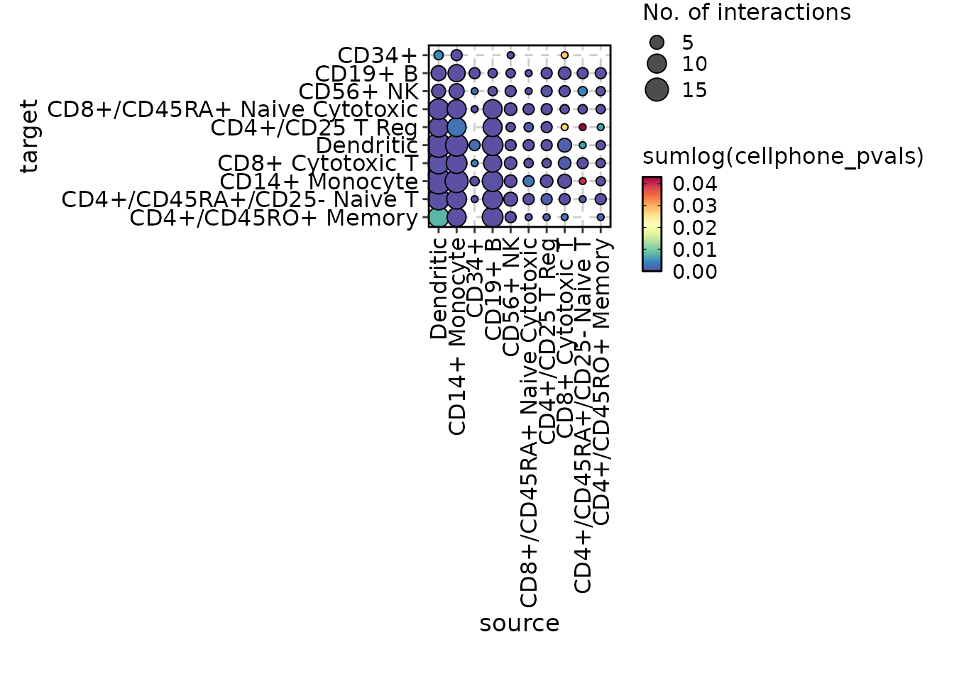
To only debug a single conversation, you can set verbose
to TRUE in the ask() method.
chat <- SCPlotterChat$new(
    provider = provider,
    verbose = FALSE
)
chat$ask("Generate a cell-cell communication plot for the cellphonedb_res data.", verbose = TRUE)
#> --- Sending request to LLM provider (deepseek-v4-flash): ---
#> Objective: Select the most appropriate tool to handle the user's request while preserving conversational context. If the user refines or changes how the previous result should be visualized (e.g., asks for a different plot type), continue with the last plotting tool used unless they explicitly name a different tool.
#>
#> Decision Process:
#> - If the user explicitly names a tool, output that tool.
#> - Else, if the request appears to refine the previous output (e.g., "do X instead", "make it a heatmap/dot/bar/etc", "change to ...", "add ... to", "same plot but ..."), select the last tool mentioned in the chat history.
#> - Else, analyze the current user request; if there is a clear, unambiguous match to a single tool, select that tool.
#> - Else, use the last mentioned tool from the chat history.
#> - If no tool is found, respond with "None".
#>
#> Response Format: Provide only the name of the selected tool, or "None" if no tool applies.
#>
#> User Request:
#> Generate a cell-cell communication plot for the cellphonedb_res data.
#>
#> Available Tools:
#> - gt: Programmatic clone selection for TCR/BCR repertoire analysis
#>    Clone selectors provide a programmatic, expression-based system for filtering
#>    and selecting T cell and B cell clones from immune repertoire data. They are
#>    the foundation of clone-level analysis in    scplotter   , enabling flexible
#>    clone selection without manual specification of clone IDs.
#>
#>    Clone selectors operate on data frames containing clone abundance information
#>    (clone IDs paired with group-level counts or fractions). They evaluate
#>    selection criteria — such as abundance thresholds, group comparisons, or
#>    shared presence across conditions — and return either the selected clone IDs,
#>    a logical indicator vector, or a filtered data frame. The system is
#>    context-aware: it automatically detects whether it is being called from
#>    within a    dplyr    pipeline, a    scplotter    function, or standalone
#>    code, and adjusts its default behavior accordingly.
#>
#>    The following selector functions are available:
#>
#>        top()    — select the    n    largest clones by abundance
#>        sel()    — select clones matching a custom logical expression
#>        uniq()    — select clones unique to a specified group
#>        shared()    — select clones present in all specified groups
#>        gt()   ,    ge()   ,    lt()   ,    le()   ,    eq()   ,    ne()    — comparison-based selection
#>        and()   ,    or()    — combine multiple selector results
#>
#>
#> - CellDimPlot: Cell Dimension Reduction Plot
#>    Visualizes single-cell data in reduced dimension space (e.g., UMAP, t-SNE,
#>    PCA). This is the primary function for exploring cell clustering, cell
#>    identity, and spatial relationships in transcriptomics datasets. It creates
#>    scatter plots where each point represents a cell, positioned by its
#>    coordinates in the reduced dimension space and colored by metadata variables
#>    such as cell type, sample condition, or cluster assignment.
#>
#>    CellDimPlot    serves as a unified interface across multiple single-cell data
#>    containers:
#>
#>        Seurat objects    — Extracts embeddings from    Reductions()    and
#>    metadata from    @meta.data   . The default reduction is auto-detected
#>    via    default_dimreduc()   .
#>        Giotto objects    — Extracts spatial dimension reductions and cell
#>    metadata using    spat_unit    and    feat_type    to identify the correct
#>    spatial unit and feature type.
#>        h5ad files    (.h5ad or opened    H5File   ) — Reads from    obsm    for
#>    embeddings and    obs    for metadata. Reduction names are automatically
#>    prefixed with    "X_"    when needed (e.g.,    "umap"    →    "X_umap"   ).
#>
#>
#>    Beyond basic cluster visualization,    CellDimPlot    supports a rich set of
#>    visual overlays and analytical enhancements:
#>
#>        Cluster highlighting    — Emphasize cells matching a logical
#>    expression while dimming others (   highlight   ).
#>        Group labels    — Add text labels at group centroids (   label   ,
#>    label_insitu   ).
#>        Group marks    — Draw boundary shapes around groups: ellipse,
#>    rectangle, or circle (   add_mark   ,    mark_type   ).
#>        Density contours    — Overlay 2D density estimates (   add_density   ).
#>        Neighbor graphs    — Draw edges between neighboring cells from
#>    k-NN or shared-nearest-neighbor graphs (   graph   ).
#>        Lineage trajectories    — Overlay pseudotime lineage curves
#>    (   lineages   ).
#>        Velocity arrows    — Overlay RNA velocity vectors on the embedding
#>    (   velocity   ). For dedicated velocity visualization with grid or
#>    stream plots, see    CellVelocityPlot   .
#>        Statistical charts    — Embed small bar, ring, or line charts at
#>    group positions showing composition of a second variable (   stat_by   ,
#>    stat_plot_type   ).
#>        Hexagonal binning    — Replace scatter points with binned hexagons
#>    for large datasets (   hex   ).
#>        3D visualization    — Plot three dimensions by specifying
#>    dims = 1:3   .
#>        Rasterization    — Render points as a raster image for performance
#>    with large cell counts (   raster   ).
#>
#>
#> - ClonalVolumePlot: Clonal Volume Plot
#>    Visualizes the number (or fraction) of unique T-cell or B-cell clones across
#>    samples and metadata groups. Clonal volume — the count of distinct clonotypes
#>    detected in a sample — is a fundamental measure of immune repertoire diversity.
#>    Higher clonal volume indicates a more diverse repertoire, while lower volume
#>    may reflect clonal expansion in response to antigen stimulation.
#>
#>    ClonalVolumePlot    computes clonal counts via
#>    scRepertoire::clonalQuant()    and
#>    visualizes them as bar, box, or violin plots. It accepts both
#>    scRepertoire    combined TCR/BCR data and Seurat objects with clonal
#>    information integrated via    scRepertoire::combineExpression()   .
#>
#> - ClonalRarefactionPlot: Clonal Rarefaction Plot
#>    Visualizes clonal rarefaction curves — estimates of clone richness as a
#>    function of sampling depth. Rarefaction addresses a fundamental challenge
#>    in immune repertoire analysis: the number of clones observed depends on
#>    how many cells are sequenced. By repeatedly subsampling (bootstrapping)
#>    the data at varying depths, rarefaction curves reveal whether the
#>    repertoire has been sampled to saturation or whether additional
#>    sequencing would uncover many more clones.
#>
#>    ClonalRarefactionPlot    extracts clone count data from the repertoire,
#>    optionally groups it by metadata columns, and generates rarefaction
#>    curves via    plotthis::RarefactionPlot()   .
#>    When    split_by    is specified, separate plots are generated for each split
#>    group and combined into a multi-panel layout.
#>
#> - ClonalStatPlot: Visualize clone abundance, frequency, and dynamics across groups
#>    ClonalStatPlot provides a unified interface for visualizing the abundance, frequency,
#>    and dynamics of T cell and B cell clones across experimental groups. It is the most
#>    versatile clone visualization function in scplotter, offering multiple plot types
#>    for different analytical purposes.
#>
#>    The function operates on the output of    scRepertoire::combineTCR()   ,
#>    scRepertoire::combineBCR()   , or
#>    scRepertoire::combineExpression()   . Clones are
#>    identified by their CDR3 amino acid sequence, nucleotide sequence, V(D)J gene usage,
#>    or a combination thereof (via    clone_call   ). The function then computes clone-level
#>    statistics (size, fraction, or count of clones) within each group and renders them
#>    using one of ten supported plot types.
#>
#>    A defining feature of ClonalStatPlot is its flexible clone selection system. Clones
#>    can be specified directly by their IDs, or selected programmatically using expression
#>    selectors such as    top()   ,    sel()   ,    shared()   ,    uniq()   , and
#>    comparison operators (   gt()   ,    lt()   ,    eq()   , etc.). These selectors
#>    evaluate within the context of each faceting/splitting group, enabling per-group
#>    selection of the most expanded clones, clones shared between conditions, or clones
#>    meeting custom abundance thresholds. See the    Clone selection    section below
#>    and    CloneSelectors    for full details.
#>
#>    Clones can also be aggregated into named groups (by passing a named list to
#>    clones   ), where each group is defined by its own selection expression. In
#>    this mode, the visualization unit becomes the clone group rather than individual
#>    clones, enabling comparisons such as "hyper-expanded clones in condition A" vs.
#>    "hyper-expanded clones in condition B."
#>
#> - ClonalCompositionPlot: Clonal Composition Plot
#>    Visualizes the composition of the immune repertoire by categorizing clones
#>    into abundance groups (Rare, Small, Medium, Large, Hyperexpanded) and
#>    plotting their relative proportions across samples or metadata groups.
#>    This reveals the overall structure of the repertoire — whether it is
#>    dominated by a few large clones (clonal expansion) or composed of many
#>    small clones (high diversity).
#>
#>    ClonalCompositionPlot    supports three analysis methods:
#>
#>        Homeostasis    (   "homeostasis"   ,    "homeo"   ,    "rel"   ) —
#>    Clones are binned by their frequency (fraction of the total
#>    repertoire) into categories such as Rare, Small, Medium, Large,
#>    and Hyperexpanded. Uses
#>    scRepertoire::clonalHomeostasis()   .
#>        Top clones    (   "top"   ) — Clones are ranked and binned by
#>    their rank index (e.g., top 10, top 100, etc.). Uses
#>    scRepertoire::clonalProportion()   .
#>        Rare clones    (   "rare"   ) — Clones are binned by their
#>    absolute size (clone count). Uses clone size thresholds directly.
#>
#>
#> - EnrichmentPlot: Visualize gene set enrichment and over-representation analysis results
#>    Gene set enrichment analysis identifies biological pathways, gene ontologies,
#>    or functional categories that are statistically over-represented among a list
#>    of genes of interest (e.g., differentially expressed genes from a single-cell
#>    RNA-seq experiment). Rather than interpreting individual genes in isolation,
#>    enrichment analysis places gene-level results into a broader biological context,
#>    revealing which processes, functions, or diseases are perturbed.
#>
#>    EnrichmentPlot    generates publication-quality visualizations for enrichment
#>    results across eight distinct plot types, each suited to a different analytical
#>    perspective:
#>
#>        bar    — Horizontal bar chart of the top enriched terms, ordered by
#>    significance. Best for a quick overview or when showing a small number of terms.
#>        dot    — Dot plot where x-axis shows a continuous metric (default:
#>    GeneRatio   ), dot size reflects gene count, and dot color reflects
#>    significance. Ideal for comparing terms along two dimensions simultaneously.
#>        lollipop    — Lollipop chart combining dot and bar aesthetics.
#>    Similar to the dot plot but with stems emphasizing the ranking.
#>        comparison    — Side-by-side dot plot comparing enrichment across
#>    groups (e.g., cell types, conditions). Requires    group_by   .
#>        network    — Network visualization where nodes are enriched terms
#>    and edges represent overlapping gene sets. Reveals functional modules and
#>    redundant terms.
#>        enrichmap    — Enrichment map similar to the network plot but
#>    optimized for large term sets (default    top_term = 100   ). Nodes are
#>    terms and edges represent gene overlap.
#>        wordcloud    — Word cloud where term size reflects significance.
#>    Can display either enrichment terms (   word_type = "term"   ) or
#>    individual gene symbols (   word_type = "feature"   ).
#>        heatmap    — Heatmap of enrichment significance across groups
#>    (   group_by    is mapped to columns). Useful for comparing enrichment
#>    patterns across multiple conditions or cell types.
#>
#>
#>    The function auto-detects the input data format (   clusterProfiler    or
#>    enrichR   ) and delegates visualization to the appropriate    plotthis
#>    plotting function.
#>
#> - eq: Programmatic clone selection for TCR/BCR repertoire analysis
#>    Clone selectors provide a programmatic, expression-based system for filtering
#>    and selecting T cell and B cell clones from immune repertoire data. They are
#>    the foundation of clone-level analysis in    scplotter   , enabling flexible
#>    clone selection without manual specification of clone IDs.
#>
#>    Clone selectors operate on data frames containing clone abundance information
#>    (clone IDs paired with group-level counts or fractions). They evaluate
#>    selection criteria — such as abundance thresholds, group comparisons, or
#>    shared presence across conditions — and return either the selected clone IDs,
#>    a logical indicator vector, or a filtered data frame. The system is
#>    context-aware: it automatically detects whether it is being called from
#>    within a    dplyr    pipeline, a    scplotter    function, or standalone
#>    code, and adjusts its default behavior accordingly.
#>
#>    The following selector functions are available:
#>
#>        top()    — select the    n    largest clones by abundance
#>        sel()    — select clones matching a custom logical expression
#>        uniq()    — select clones unique to a specified group
#>        shared()    — select clones present in all specified groups
#>        gt()   ,    ge()   ,    lt()   ,    le()   ,    eq()   ,    ne()    — comparison-based selection
#>        and()   ,    or()    — combine multiple selector results
#>
#>
#> - CellVelocityPlot: Cell Velocity Plot
#>    Visualizes RNA velocity on a reduced-dimension embedding. RNA velocity
#>    infers the future transcriptional state of individual cells by modeling the
#>    ratio of unspliced (nascent) to spliced (mature) mRNA transcripts. On a
#>    dimension reduction plot, velocity is displayed as arrows (or grid/stream
#>    fields) showing the predicted direction and magnitude of transcriptional
#>    change for each cell — effectively revealing the "flow" of cells through
#>    differentiation, development, or other state transitions.
#>
#>    CellVelocityPlot    serves as a unified interface across multiple single-cell
#>    data containers:
#>
#>        Seurat objects    — Extracts embeddings from both the main
#>    reduction (   reduction   ) and the velocity reduction
#>    (   v_reduction   ) via    Embeddings()   ; metadata for grouping via
#>    @meta.data   .
#>        Giotto objects    — Extracts dimension reductions via
#>    getDimReduction()    using    spat_unit    and    feat_type    to identify
#>    the correct spatial unit and feature type.
#>        h5ad files    (.h5ad or opened    H5File   ) — Reads from    obsm    for
#>    both the main and velocity embeddings;    obs    for metadata. Reduction
#>    names are automatically prefixed with    "X_"    when needed.
#>
#>
#> - SpatFeaturePlot: Visualize feature expression on spatial coordinates
#>    Plot continuous feature values — gene expression, dimension reduction
#>    components, metadata columns, or any numeric variable — directly on
#>    spatial tissue coordinates.    SpatFeaturePlot()    is the spatial
#>    analogue of a feature plot over a UMAP/t-SNE embedding: it paints each
#>    spot, cell, or molecule with the expression level of one or more features,
#>    revealing the spatial organization of gene activity.
#>
#>    Multiple features are automatically faceted, making it easy to compare
#>    spatial expression patterns across a gene panel in a single plot. For
#>    categorical grouping (e.g., cluster identity on spatial coordinates), use
#>    SpatDimPlot    instead.
#>
#> - shared: Programmatic clone selection for TCR/BCR repertoire analysis
#>    Clone selectors provide a programmatic, expression-based system for filtering
#>    and selecting T cell and B cell clones from immune repertoire data. They are
#>    the foundation of clone-level analysis in    scplotter   , enabling flexible
#>    clone selection without manual specification of clone IDs.
#>
#>    Clone selectors operate on data frames containing clone abundance information
#>    (clone IDs paired with group-level counts or fractions). They evaluate
#>    selection criteria — such as abundance thresholds, group comparisons, or
#>    shared presence across conditions — and return either the selected clone IDs,
#>    a logical indicator vector, or a filtered data frame. The system is
#>    context-aware: it automatically detects whether it is being called from
#>    within a    dplyr    pipeline, a    scplotter    function, or standalone
#>    code, and adjusts its default behavior accordingly.
#>
#>    The following selector functions are available:
#>
#>        top()    — select the    n    largest clones by abundance
#>        sel()    — select clones matching a custom logical expression
#>        uniq()    — select clones unique to a specified group
#>        shared()    — select clones present in all specified groups
#>        gt()   ,    ge()   ,    lt()   ,    le()   ,    eq()   ,    ne()    — comparison-based selection
#>        and()   ,    or()    — combine multiple selector results
#>
#>
#> - CellStatPlot: Cell statistics plot
#>    Visualizes cell-level statistics — counts, fractions, and composition —
#>    across cell identities and metadata groupings. This is the primary function
#>    for exploring the distribution of cell types, clusters, and categorical
#>    metadata in single-cell transcriptomics datasets. It answers questions such
#>    as: "What proportion of each cell type is in each condition?", "How do
#>    cluster abundances change across samples?", and "What is the clonal
#>    composition within each cell type?"
#>
#>    CellStatPlot    serves as a unified interface across 15+ visualization
#>    types, all driven by a common data aggregation and fraction-calculation
#>    pipeline. It supports four single-cell data containers:
#>
#>        Seurat objects    — Extracts    @meta.data   ; uses    Idents()    as
#>    the default identity when    ident = NULL   .
#>        Giotto objects    — Extracts cell metadata via
#>    getCellMetadata()    using    spat_unit    and    feat_type   .
#>        h5ad files    (.h5ad or opened    H5File   ) — Reads from    obs
#>    via    h5group_to_dataframe()   .
#>        Data frames    — Internal method; all other methods ultimately
#>    delegate here after metadata extraction.
#>
#>
#> - ne: Programmatic clone selection for TCR/BCR repertoire analysis
#>    Clone selectors provide a programmatic, expression-based system for filtering
#>    and selecting T cell and B cell clones from immune repertoire data. They are
#>    the foundation of clone-level analysis in    scplotter   , enabling flexible
#>    clone selection without manual specification of clone IDs.
#>
#>    Clone selectors operate on data frames containing clone abundance information
#>    (clone IDs paired with group-level counts or fractions). They evaluate
#>    selection criteria — such as abundance thresholds, group comparisons, or
#>    shared presence across conditions — and return either the selected clone IDs,
#>    a logical indicator vector, or a filtered data frame. The system is
#>    context-aware: it automatically detects whether it is being called from
#>    within a    dplyr    pipeline, a    scplotter    function, or standalone
#>    code, and adjusts its default behavior accordingly.
#>
#>    The following selector functions are available:
#>
#>        top()    — select the    n    largest clones by abundance
#>        sel()    — select clones matching a custom logical expression
#>        uniq()    — select clones unique to a specified group
#>        shared()    — select clones present in all specified groups
#>        gt()   ,    ge()   ,    lt()   ,    le()   ,    eq()   ,    ne()    — comparison-based selection
#>        and()   ,    or()    — combine multiple selector results
#>
#>
#> - SpatDimPlot: Visualize categorical groups on spatial coordinates
#>    Plot categorical metadata — cluster identities, tissue regions, sample
#>    labels, or any discrete grouping variable — directly on spatial tissue
#>    coordinates.    SpatDimPlot()    is the spatial analogue of a UMAP/t-SNE
#>    plot colored by cluster: each spot, cell, or molecule is colored by its
#>    group membership, making it easy to assess the spatial organization of
#>    cell types, anatomical regions, or experimental conditions.
#>
#>    For continuous features (gene expression, dimension reduction scores),
#>    use    SpatFeaturePlot    instead.
#>
#> - GSEASummaryPlot: Objects exported from other packages
#>    These objects are imported from other packages. Follow the links
#>    below to see their documentation.
#>
#>
#>         plotthis   GSEAPlot()   ,    GSEASummaryPlot()
#>
#> - CCCPlot: Visualize Cell-Cell Communication (CCC) Interactions
#>    Cell-cell communication (CCC) is the process by which cells send and receive
#>    molecular signals — typically through ligand-receptor (LR) interactions — to
#>    coordinate tissue function. CCC analysis infers these interactions from
#>    single-cell transcriptomics data by identifying which ligand-receptor pairs
#>    are expressed between which cell types, often scoring each interaction by
#>    its magnitude (e.g., expression level, interaction score) and specificity
#>    (e.g., a p-value quantifying how cell-type-specific the interaction is).
#>
#>    CCCPlot    provides a unified interface to visualize CCC inference results
#>    (from tools like CellPhoneDB, LIANA, CellChat, NicheNet, etc.) across many
#>    plot types. It supports two fundamental modes:
#>
#>    Aggregation mode    (   method = "aggregation"   , the default): Ligand-receptor
#>    pairs are aggregated per source-target cell type pair. This shows    which
#>    cell types communicate    and how strongly. Supported plot types:    "network"   ,
#>    "chord"   /   "circos"   ,    "heatmap"   ,    "sankey"   /   "alluvial"   ,    "dot"   .
#>
#>    Interaction mode    (   method = "interaction"   ): Individual ligand-receptor
#>    pairs are plotted. This shows    which specific LR pairs    mediate the
#>    communication. Supported plot types:    "dot"   ,    "network"   ,    "heatmap"   ,
#>    "box"   ,    "violin"   ,    "ridge"   .
#>
#>    The    "linkedheatmap"    plot type is a special case: it does not use the
#>    method    parameter. It displays a side-by-side heatmap where the left side
#>    shows ligand expression across source cell types and the right side shows
#>    receptor expression across target cell types, with links between them
#>    representing the LR pairs. This plot type requires    ligand_means    and
#>    receptor_means    columns.
#>
#>    Under the hood,    CCCPlot    preprocesses the data (aggregating or
#>    reformatting as needed) and delegates rendering to the corresponding
#>    plotthis    package function. All styling and layout arguments accepted by
#>    those functions can be passed through    ...   .
#>
#> - ClonalResidencyPlot: Clonal Residency Plot
#>    Visualizes the sharing (residency) of T-cell or B-cell clones across
#>    different samples or metadata groups. Clonal residency analysis reveals
#>    how clonotypes are distributed — whether a clone is private to one
#>    condition or shared across multiple conditions — which is critical for
#>    understanding immune responses, tracking antigen-specific clones, and
#>    identifying public vs. private repertoires.
#>
#>    ClonalResidencyPlot    supports three visualization modes:
#>
#>        Scatter plot    — Compares clone sizes between two groups on
#>    log-transformed axes. Points are colored by clonal category:
#>    singletons (unique to one group), expanded clones, and dual
#>    clones (shared between groups). Correlation statistics are
#>    displayed in the subtitle.
#>        Venn diagram    — Shows the overlap of clone sets between up
#>    to 4 groups. When    with_class = TRUE   , labels include singlet
#>    counts.
#>        UpSet plot    — Shows intersection sizes for any number of
#>    groups. When    with_class = TRUE   , clone classes (singlet,
#>    expanded) are displayed as separate intersections.
#>
#>
#> - ClustreePlot: Visualize cluster stability across clustering resolutions
#>    A clustree plot visualizes how cells move between clusters when clustering is
#>    performed at different resolutions. Each resolution level is a column of nodes,
#>    and edges show the flow of cells between clusters at adjacent resolutions.
#>    This is an essential diagnostic for single-cell analysis, helping researchers
#>    choose an appropriate clustering resolution by revealing which clusters are
#>    stable (persistent across resolutions) and which are transient (appear only at
#>    specific resolutions).
#>
#>    This function is a wrapper around    plotthis::ClustreePlot()
#>    that automatically extracts the metadata from Seurat objects. For data frames,
#>    the data is passed directly to    plotthis   .
#>
#> - ClonalKmerPlot: Visualize CDR3 k-mer (motif) frequency
#>    Short amino acid motifs within CDR3 sequences — termed    k-mers    — can reveal
#>    shared binding specificities, common structural elements, and repertoire-level
#>    sequence features that are not apparent from full-length sequence analysis
#>    alone. Specific k-mers may be enriched in responses to particular antigens,
#>    represent public TCR/BCR motifs shared across individuals, or reflect
#>    convergent recombination events.
#>
#> - ClonalPositionalPlot: Visualize positional properties of CDR3 sequences
#>    The complementarity-determining region 3 (CDR3) is the most variable region of
#>    T cell and B cell receptors, and is the primary determinant of antigen
#>    specificity. Analyzing how amino acid composition, diversity, and
#>    physicochemical properties vary across CDR3 positions provides insight into
#>    repertoire structure, selection pressures, and the biophysical constraints
#>    that shape antigen recognition.
#>
#> - uniq: Programmatic clone selection for TCR/BCR repertoire analysis
#>    Clone selectors provide a programmatic, expression-based system for filtering
#>    and selecting T cell and B cell clones from immune repertoire data. They are
#>    the foundation of clone-level analysis in    scplotter   , enabling flexible
#>    clone selection without manual specification of clone IDs.
#>
#>    Clone selectors operate on data frames containing clone abundance information
#>    (clone IDs paired with group-level counts or fractions). They evaluate
#>    selection criteria — such as abundance thresholds, group comparisons, or
#>    shared presence across conditions — and return either the selected clone IDs,
#>    a logical indicator vector, or a filtered data frame. The system is
#>    context-aware: it automatically detects whether it is being called from
#>    within a    dplyr    pipeline, a    scplotter    function, or standalone
#>    code, and adjusts its default behavior accordingly.
#>
#>    The following selector functions are available:
#>
#>        top()    — select the    n    largest clones by abundance
#>        sel()    — select clones matching a custom logical expression
#>        uniq()    — select clones unique to a specified group
#>        shared()    — select clones present in all specified groups
#>        gt()   ,    ge()   ,    lt()   ,    le()   ,    eq()   ,    ne()    — comparison-based selection
#>        and()   ,    or()    — combine multiple selector results
#>
#>
#> - top: Programmatic clone selection for TCR/BCR repertoire analysis
#>    Clone selectors provide a programmatic, expression-based system for filtering
#>    and selecting T cell and B cell clones from immune repertoire data. They are
#>    the foundation of clone-level analysis in    scplotter   , enabling flexible
#>    clone selection without manual specification of clone IDs.
#>
#>    Clone selectors operate on data frames containing clone abundance information
#>    (clone IDs paired with group-level counts or fractions). They evaluate
#>    selection criteria — such as abundance thresholds, group comparisons, or
#>    shared presence across conditions — and return either the selected clone IDs,
#>    a logical indicator vector, or a filtered data frame. The system is
#>    context-aware: it automatically detects whether it is being called from
#>    within a    dplyr    pipeline, a    scplotter    function, or standalone
#>    code, and adjusts its default behavior accordingly.
#>
#>    The following selector functions are available:
#>
#>        top()    — select the    n    largest clones by abundance
#>        sel()    — select clones matching a custom logical expression
#>        uniq()    — select clones unique to a specified group
#>        shared()    — select clones present in all specified groups
#>        gt()   ,    ge()   ,    lt()   ,    le()   ,    eq()   ,    ne()    — comparison-based selection
#>        and()   ,    or()    — combine multiple selector results
#>
#>
#> - le: Programmatic clone selection for TCR/BCR repertoire analysis
#>    Clone selectors provide a programmatic, expression-based system for filtering
#>    and selecting T cell and B cell clones from immune repertoire data. They are
#>    the foundation of clone-level analysis in    scplotter   , enabling flexible
#>    clone selection without manual specification of clone IDs.
#>
#>    Clone selectors operate on data frames containing clone abundance information
#>    (clone IDs paired with group-level counts or fractions). They evaluate
#>    selection criteria — such as abundance thresholds, group comparisons, or
#>    shared presence across conditions — and return either the selected clone IDs,
#>    a logical indicator vector, or a filtered data frame. The system is
#>    context-aware: it automatically detects whether it is being called from
#>    within a    dplyr    pipeline, a    scplotter    function, or standalone
#>    code, and adjusts its default behavior accordingly.
#>
#>    The following selector functions are available:
#>
#>        top()    — select the    n    largest clones by abundance
#>        sel()    — select clones matching a custom logical expression
#>        uniq()    — select clones unique to a specified group
#>        shared()    — select clones present in all specified groups
#>        gt()   ,    ge()   ,    lt()   ,    le()   ,    eq()   ,    ne()    — comparison-based selection
#>        and()   ,    or()    — combine multiple selector results
#>
#>
#> - MarkersPlot: Visualize differential expression markers
#>    Visualize differential expression (DE) results — typically the output of
#>    Seurat::FindMarkers()    or
#>    Seurat::FindAllMarkers()    — across a
#>    variety of plot types. You can also compose the DE results from other
#>    tools into a data frame with the required columns and use this function to visualize them.
#>
#>    MarkersPlot()    bridges the gap between DE
#>    testing and visualization by providing a unified interface for both
#>    summary-level DE visualizations    (volcano, jitter, heatmap, and dot
#>    plots of fold changes and significance) and    expression-level
#>    visualizations    (violin, box, bar, ridge, heatmap, and dot plots of actual
#>    expression values from a Seurat object).
#>
#>    The function handles two broad categories of plots:
#>
#>        DE summary plots    (no    object    required): visualize the
#>    DE statistics themselves — log2 fold change, percentage difference,
#>    p-values, and adjusted p-values — across groups or comparisons.
#>
#>        "volcano"    /    "volcano_log2fc"    — Volcano plot with
#>    log2 fold change on the x-axis and    -log_{10}(p)    on the y-axis.
#>    Genes passing the    cutoff    are highlighted and top genes are
#>    labeled. Ideal for overview of effect size vs. significance.
#>        "volcano_pct"    — Volcano plot with percentage-point
#>    difference (   pct.1 - pct.2   ) on the x-axis. Useful when the
#>    biological question is about detection rate rather than expression
#>    magnitude.
#>        "jitter"    /    "jitter_log2fc"    — Jitter plot of log2
#>    fold changes across groups (defined by    each   ). Dot size
#>    encodes    -log_{10}(p)   . Reveals distribution of effect sizes
#>    per cluster or condition.
#>        "jitter_pct"    — Jitter plot of percentage-point
#>    differences across groups.
#>        "heatmap_log2fc"    — Heatmap of log2 fold changes (genes
#>    × groups). Cells can be marked for significance via    cutoff
#>    and    sig_mark   .
#>        "heatmap_pct"    — Heatmap of percentage-point differences
#>    (genes × groups). Same significance-marking support.
#>        "dot_log2fc"    — Dot plot of log2 fold changes (genes ×
#>    groups). Dot size encodes    -log_{10}(p)   .
#>        "dot_pct"    — Dot plot of percentage-point differences
#>    (genes × groups). Dot size encodes    -log_{10}(p)   .
#>
#>        Expression plots    (   object    required): visualize the
#>    actual expression values of the selected marker genes in the context of
#>    the original Seurat object. These are useful for validating DE results
#>    by inspecting the underlying expression distributions.
#>
#>        "heatmap"    — Expression heatmap of selected marker genes.
#>        "violin"    — Violin plots of expression per gene.
#>        "box"    — Box plots of expression per gene.
#>        "bar"    — Bar plots of mean expression per gene.
#>        "ridge"    — Ridge plots of expression distribution per gene.
#>        "dot"    — Dot plot of expression (fraction expressing ×
#>    mean expression) per gene.
#>
#>
#>
#> - ClonalOverlapPlot: Clonal Overlap Plot
#>    Visualizes the overlap (sharing) of T-cell or B-cell clonotypes between
#>    samples or metadata groups as a heatmap. Each cell in the heatmap
#>    quantifies the degree of clonal sharing between two groups, using one of
#>    several similarity or overlap metrics. This is a key analysis for
#>    identifying public clones shared across individuals, tracking
#>    antigen-specific clones across time points or tissues, and comparing
#>    repertoire similarity between conditions.
#>
#>    ClonalOverlapPlot    computes pairwise overlap via
#>    scRepertoire::clonalOverlap()
#>    and visualizes the resulting matrix as a labeled heatmap using
#>    plotthis::Heatmap()   .
#>
#> - ge: Programmatic clone selection for TCR/BCR repertoire analysis
#>    Clone selectors provide a programmatic, expression-based system for filtering
#>    and selecting T cell and B cell clones from immune repertoire data. They are
#>    the foundation of clone-level analysis in    scplotter   , enabling flexible
#>    clone selection without manual specification of clone IDs.
#>
#>    Clone selectors operate on data frames containing clone abundance information
#>    (clone IDs paired with group-level counts or fractions). They evaluate
#>    selection criteria — such as abundance thresholds, group comparisons, or
#>    shared presence across conditions — and return either the selected clone IDs,
#>    a logical indicator vector, or a filtered data frame. The system is
#>    context-aware: it automatically detects whether it is being called from
#>    within a    dplyr    pipeline, a    scplotter    function, or standalone
#>    code, and adjusts its default behavior accordingly.
#>
#>    The following selector functions are available:
#>
#>        top()    — select the    n    largest clones by abundance
#>        sel()    — select clones matching a custom logical expression
#>        uniq()    — select clones unique to a specified group
#>        shared()    — select clones present in all specified groups
#>        gt()   ,    ge()   ,    lt()   ,    le()   ,    eq()   ,    ne()    — comparison-based selection
#>        and()   ,    or()    — combine multiple selector results
#>
#>
#> - ClonalLengthPlot: Clonal CDR3 Length Plot
#>    Visualizes the distribution of CDR3 sequence lengths across the immune
#>    repertoire. CDR3 length is a key feature of T-cell and B-cell receptor
#>    diversity — different clones have different CDR3 lengths, and shifts in
#>    length distribution can indicate clonal selection, antigen-specific
#>    expansion, or repertoire bias.
#>
#>    ClonalLengthPlot    computes CDR3 length data via
#>    scRepertoire::clonalLength()    and
#>    visualizes the distribution as bar, box, violin, or density plots. Length
#>    is measured in amino acids (when    clone_call = "aa"   ) or nucleotides
#>    (when    clone_call = "nt"   ).
#>
#> - and: Programmatic clone selection for TCR/BCR repertoire analysis
#>    Clone selectors provide a programmatic, expression-based system for filtering
#>    and selecting T cell and B cell clones from immune repertoire data. They are
#>    the foundation of clone-level analysis in    scplotter   , enabling flexible
#>    clone selection without manual specification of clone IDs.
#>
#>    Clone selectors operate on data frames containing clone abundance information
#>    (clone IDs paired with group-level counts or fractions). They evaluate
#>    selection criteria — such as abundance thresholds, group comparisons, or
#>    shared presence across conditions — and return either the selected clone IDs,
#>    a logical indicator vector, or a filtered data frame. The system is
#>    context-aware: it automatically detects whether it is being called from
#>    within a    dplyr    pipeline, a    scplotter    function, or standalone
#>    code, and adjusts its default behavior accordingly.
#>
#>    The following selector functions are available:
#>
#>        top()    — select the    n    largest clones by abundance
#>        sel()    — select clones matching a custom logical expression
#>        uniq()    — select clones unique to a specified group
#>        shared()    — select clones present in all specified groups
#>        gt()   ,    ge()   ,    lt()   ,    le()   ,    eq()   ,    ne()    — comparison-based selection
#>        and()   ,    or()    — combine multiple selector results
#>
#>
#> - ClonalAbundancePlot: Clonal Abundance Plot
#>    Visualizes the distribution of clonal abundances — how many clones are
#>    present at each abundance level (frequency) in the repertoire. Clonal
#>    abundance distributions typically follow a power-law pattern: a small
#>    number of highly expanded clones and a large number of rare clones.
#>    This function helps characterize repertoire structure by showing whether
#>    the immune response is dominated by a few large clones (clonal expansion)
#>    or evenly distributed across many clones (high diversity).
#>
#>    ClonalAbundancePlot    computes clonal abundance data via
#>    scRepertoire::clonalAbundance()
#>    and visualizes it as trend lines, histograms, or density curves.
#>
#> - sel: Programmatic clone selection for TCR/BCR repertoire analysis
#>    Clone selectors provide a programmatic, expression-based system for filtering
#>    and selecting T cell and B cell clones from immune repertoire data. They are
#>    the foundation of clone-level analysis in    scplotter   , enabling flexible
#>    clone selection without manual specification of clone IDs.
#>
#>    Clone selectors operate on data frames containing clone abundance information
#>    (clone IDs paired with group-level counts or fractions). They evaluate
#>    selection criteria — such as abundance thresholds, group comparisons, or
#>    shared presence across conditions — and return either the selected clone IDs,
#>    a logical indicator vector, or a filtered data frame. The system is
#>    context-aware: it automatically detects whether it is being called from
#>    within a    dplyr    pipeline, a    scplotter    function, or standalone
#>    code, and adjusts its default behavior accordingly.
#>
#>    The following selector functions are available:
#>
#>        top()    — select the    n    largest clones by abundance
#>        sel()    — select clones matching a custom logical expression
#>        uniq()    — select clones unique to a specified group
#>        shared()    — select clones present in all specified groups
#>        gt()   ,    ge()   ,    lt()   ,    le()   ,    eq()   ,    ne()    — comparison-based selection
#>        and()   ,    or()    — combine multiple selector results
#>
#>
#> - ClonalDiversityPlot: Clonal Diversity Plot
#>    Visualizes clonal diversity metrics across samples or metadata groups.
#>    Clonal diversity quantifies the richness and evenness of the immune
#>    repertoire — how many distinct clonotypes are present and how evenly
#>    cells are distributed among them. High diversity indicates a broad,
#>    well-distributed repertoire; low diversity may indicate clonal expansion
#>    (oligoclonality) in response to antigen stimulation or disease.
#>
#>    ClonalDiversityPlot    computes diversity scores using a custom
#>    implementation that wraps several    scRepertoire    methods and adds
#>    three    scplotter   -specific metrics (Gini coefficient, D50, DXX).
#>    Results are visualized as bar, box, or violin plots.
#>
#> - FeatureStatPlot: Visualize feature expression and statistics across cell groups
#>    A central question in single-cell analysis is how features — genes, gene
#>    signatures, module scores, or other molecular measurements — vary across cell
#>    types, conditions, or experimental groups.    FeatureStatPlot    answers this
#>    question by providing eight complementary visualization types, each suited to
#>    a different analytical perspective:
#>
#>        violin    — Violin plot showing the full distribution of feature
#>    values per identity group. Best for comparing expression distributions
#>    and detecting bimodality or outliers.
#>        box    — Box plot summarizing feature values with quartiles and
#>    outliers. A compact alternative to the violin plot.
#>        bar    — Bar chart of aggregated feature values (default: mean)
#>    per group. Useful for summary-level comparisons with error bars.
#>        ridge    — Ridge (joy) plot showing density curves per group.
#>    Effective when comparing many groups or when distribution shape matters.
#>        dim    — Dimensionality reduction plot (UMAP, t-SNE, PCA) with
#>    cells colored by feature expression. Reveals spatial patterns of gene
#>    expression in the reduced space.
#>        cor    — Correlation plot between two features (scatter with
#>    fitted line and annotations) or among multiple features (pairs plot).
#>    Reveals co-expression relationships.
#>        heatmap    — Heatmap of feature expression across identity
#>    groups. Supports rich annotations (row/column metadata, bar charts,
#>    pie charts, violin plots) and flexible clustering. The go-to choice
#>    for visualizing many features across many groups.
#>        dot    — Dot plot (a shortcut for heatmap with
#>    cell_type = "dot"   ) where dot size reflects the fraction of
#>    expressing cells and dot color reflects mean expression. A compact,
#>    publication-ready format for marker gene visualization.
#>
#>
#>    The function is an S3 generic with methods for    Seurat    objects,
#>    Giotto    objects, AnnData (.h5ad) file paths, and    H5File    objects
#>    (via    hdf5r   ). Each method extracts the relevant expression matrix and
#>    metadata, then delegates to the internal    .feature_stat_plot()    which
#>    dispatches to the appropriate    plotthis    plotting function.
#>
#> - ClonalGeneUsagePlot: Visualize TCR/BCR gene segment usage
#>    Adaptive immune receptors (TCRs and BCRs) are assembled through V(D)J recombination,
#>    where variable (V), diversity (D), and joining (J) gene segments are randomly selected
#>    and rearranged. The frequency with which different gene segments are used — termed
#>    gene usage    — provides insight into immune repertoire composition, T/B cell
#>    development, and antigen-driven selection. Skewed gene usage can indicate clonal
#>    expansion, immune aging, or disease-associated repertoire bias.
#>
#> - lt: Programmatic clone selection for TCR/BCR repertoire analysis
#>    Clone selectors provide a programmatic, expression-based system for filtering
#>    and selecting T cell and B cell clones from immune repertoire data. They are
#>    the foundation of clone-level analysis in    scplotter   , enabling flexible
#>    clone selection without manual specification of clone IDs.
#>
#>    Clone selectors operate on data frames containing clone abundance information
#>    (clone IDs paired with group-level counts or fractions). They evaluate
#>    selection criteria — such as abundance thresholds, group comparisons, or
#>    shared presence across conditions — and return either the selected clone IDs,
#>    a logical indicator vector, or a filtered data frame. The system is
#>    context-aware: it automatically detects whether it is being called from
#>    within a    dplyr    pipeline, a    scplotter    function, or standalone
#>    code, and adjusts its default behavior accordingly.
#>
#>    The following selector functions are available:
#>
#>        top()    — select the    n    largest clones by abundance
#>        sel()    — select clones matching a custom logical expression
#>        uniq()    — select clones unique to a specified group
#>        shared()    — select clones present in all specified groups
#>        gt()   ,    ge()   ,    lt()   ,    le()   ,    eq()   ,    ne()    — comparison-based selection
#>        and()   ,    or()    — combine multiple selector results
#>
#>
#> - GSEAPlot: Objects exported from other packages
#>    These objects are imported from other packages. Follow the links
#>    below to see their documentation.
#>
#>
#>         plotthis   GSEAPlot()   ,    GSEASummaryPlot()
#>
#> - or: Programmatic clone selection for TCR/BCR repertoire analysis
#>    Clone selectors provide a programmatic, expression-based system for filtering
#>    and selecting T cell and B cell clones from immune repertoire data. They are
#>    the foundation of clone-level analysis in    scplotter   , enabling flexible
#>    clone selection without manual specification of clone IDs.
#>
#>    Clone selectors operate on data frames containing clone abundance information
#>    (clone IDs paired with group-level counts or fractions). They evaluate
#>    selection criteria — such as abundance thresholds, group comparisons, or
#>    shared presence across conditions — and return either the selected clone IDs,
#>    a logical indicator vector, or a filtered data frame. The system is
#>    context-aware: it automatically detects whether it is being called from
#>    within a    dplyr    pipeline, a    scplotter    function, or standalone
#>    code, and adjusts its default behavior accordingly.
#>
#>    The following selector functions are available:
#>
#>        top()    — select the    n    largest clones by abundance
#>        sel()    — select clones matching a custom logical expression
#>        uniq()    — select clones unique to a specified group
#>        shared()    — select clones present in all specified groups
#>        gt()   ,    ge()   ,    lt()   ,    le()   ,    eq()   ,    ne()    — comparison-based selection
#>        and()   ,    or()    — combine multiple selector results
#>
#>
#> - ListTools: List all available tools
#> List all available tools that can be used to handle the chat request.
#>
#> - ListData: List all available data objects
#> List all available data objects that can be used to handle the chat request.
#> --- Receiving response from LLM provider: ---
#> CCCPlot
#> Tool identified:  CCCPlot
#> --- Sending request to LLM provider (deepseek-v4-flash): ---
#> Objective: Identify the data object to be used.
#>
#> Decision Process:
#> - If the user explicitly names a data object, output that data object name. If the name does not match exactly the available ones, use the one that is mostly related.
#> - Else, if the request appears to refine the previous output (e.g., "do X instead", "make it a heatmap/dot/bar/etc", "change to ...", "add ... to", "same plot but ..."), select the last dataset name mentioned in the chat history.
#> - Else, analyze the current user request; if there is a clear, unambiguous match to a dataset, select that data object.
#> - Else, use the last mentioned data object from the chat history.
#> - If no data object is found, respond with "None".
#>
#> Response Format: Provide only the name of the selected data object, or "None" if no tool applies. The response should be unquoted.
#>
#> User Request:
#> Generate a cell-cell communication plot for the cellphonedb_res data.
#>
#> Available Data Objects:
#> - scplotter::cellphonedb_res: A toy example of CellPhoneDB output from LIANA
#> - scplotter::ifnb_sub: A subsetted version of 'ifnb' datasets
#> - scplotter::pancreas_sub: A subsetted version of mouse 'pancreas' datasets
#> - Seurat::cc.genes: Cell cycle genes
#> - Seurat::cc.genes.updated.2019: Cell cycle genes: 2019 update
#> - SeuratObject::pbmc_small: A small example version of the PBMC dataset
#> - scRepertoire::contig_list: A list of 8 single-cell T cell receptor sequences runs.
#> - scRepertoire::mini_contig_list: Processed subset of 'contig_list'
#> - scRepertoire::scRep_example: A Seurat object of 500 single T cells,
#> --- Receiving response from LLM provider: ---
#> scplotter::cellphonedb_res
#> Data object identified:  scplotter::cellphonedb_res
#> Warning in wrap$modify_fn(prompt_text, llm_provider): The 'skimr' package is
#> required to skim dataframes. Skim summary of dataframes currently not shown in
#> prompt
#> --- Sending request to LLM provider (deepseek-v4-flash): ---
#> Objective: Generate the R code to run the specified tool using the specified data object based on the user's request and the provided tool information.
#>
#> Decision Process:
#> - Analyze the user's request to understand what needs to be done with the specified tool and data object.
#> - When use the data object name, do not quote it.
#> - Refer to the provided tool information to understand the tool's usage, arguments, and examples.
#> - Consider any specific parameters or options mentioned in the user's request that need to be included in the tool call.
#> - If the user's request is ambiguous or lacks necessary details, refer to the chat history for additional context that may help clarify the intended use of the tool and data object.
#> - Construct the R code that correctly calls the tool with the specified data object, ensuring that all necessary arguments are included and correctly formatted.
#>
#> Response Format: Provide only the valid R code wrapped between "```r" and "```" to run the tool.
#>
#> Tool to be used: CCCPlot
#> Data object to be used: cellphonedb_res
#>
#> User Request:
#> Generate a cell-cell communication plot for the cellphonedb_res data.
#>
#> Tool Information:
#> - title
#> Visualize Cell-Cell Communication (CCC) Interactions
#> - description
#>
#> Cell-cell communication (CCC) is the process by which cells send and receive
#> molecular signals — typically through ligand-receptor (LR) interactions — to
#> coordinate tissue function. CCC analysis infers these interactions from
#> single-cell transcriptomics data by identifying which ligand-receptor pairs
#> are expressed between which cell types, often scoring each interaction by
#> its magnitude (e.g., expression level, interaction score) and specificity
#> (e.g., a p-value quantifying how cell-type-specific the interaction is).
#>
#> CCCPlot provides a unified interface to visualize CCC inference results
#> (from tools like CellPhoneDB, LIANA, CellChat, NicheNet, etc.) across many
#> plot types. It supports two fundamental modes:
#>
#> Aggregation mode ( method = "aggregation" , the default): Ligand-receptor
#> pairs are aggregated per source-target cell type pair. This shows which
#> cell types communicate and how strongly. Supported plot types: "network" ,
#> "chord" / "circos" , "heatmap" , "sankey" / "alluvial" , "dot" .
#>
#> Interaction mode ( method = "interaction" ): Individual ligand-receptor
#> pairs are plotted. This shows which specific LR pairs mediate the
#> communication. Supported plot types: "dot" , "network" , "heatmap" ,
#> "box" , "violin" , "ridge" .
#>
#> The "linkedheatmap" plot type is a special case: it does not use the
#> method parameter. It displays a side-by-side heatmap where the left side
#> shows ligand expression across source cell types and the right side shows
#> receptor expression across target cell types, with links between them
#> representing the LR pairs. This plot type requires ligand_means and
#> receptor_means columns.
#>
#> Under the hood, CCCPlot preprocesses the data (aggregating or
#> reformatting as needed) and delegates rendering to the corresponding
#> plotthis package function. All styling and layout arguments accepted by
#> those functions can be passed through ... .
#>
#> - usage
#>
#> CCCPlot(
#> data,
#> plot_type = c("dot", "network", "chord", "circos", "heatmap", "sankey", "alluvial",
#> "box", "violin", "ridge", "linkedheatmap"),
#> method = c("aggregation", "interaction"),
#> magnitude = waiver(),
#> specificity = waiver(),
#> ligand_expr = "ligand_means",
#> receptor_expr = "receptor_means",
#> magnitude_agg = length,
#> magnitude_name = "No. of interactions",
#> meta_specificity = "sumlog",
#> split_by = NULL,
#> x_text_angle = 90,
#> link_curvature = 0.2,
#> link_alpha = 0.6,
#> facet_by = NULL,
#> show_row_names = TRUE,
#> show_column_names = TRUE,
#> values_fill = 0,
#> right_row_dend_side = "right",
#> columns_split_by = NULL,
#> rows_split_by = NULL,
#> ...
#> )
#>
#> - arguments
#> - data: A data frame containing cell-cell communication inference
#> results. Must include the columns source, target, ligand, and
#> receptor (as character or factor). Typically also includes one or more
#> numeric columns for interaction magnitude and specificity. See the
#> Data format section above for details.
#> - plot_type: The type of visualization. Default is "dot".
#> Possible values:
#>
#> "network": Source and target cell types as nodes, interactions as
#> edges. Edge thickness encodes magnitude. Accepts link_curvature and
#> link_alpha styling. When method = "interaction", nodes are ligands
#> and receptors instead, colored by source-target pair.
#> "chord", "circos" (aliases): Chord diagram linking source and target
#> cell types. Only available with method = "aggregation".
#> "heatmap": Source cell types on rows, target cell types on columns,
#> magnitude encoded as fill color. When method = "interaction", rows are
#> individual LR pairs and columns are split by source.
#> "sankey", "alluvial" (aliases): Flow diagram from source to target
#> cell types. Only available with method = "aggregation".
#> "dot": Source vs target grid with dot size encoding magnitude and
#> (optionally) dot color encoding specificity. Available in both methods.
#> "box": Box plots of interaction strengths. Each panel is a source cell
#> type, x-axis is target cell type. Only available with
#> method = "interaction".
#> "violin": Violin plots of interaction strengths. Layout is the same as
#> "box". Only available with method = "interaction".
#> "ridge": Ridge (joy) plots of interaction strengths. Rows are target
#> cell types, faceted by source. Only available with
#> method = "interaction".
#> "linkedheatmap": Side-by-side heatmaps showing ligand expression
#> (left, by source cell types) and receptor expression (right, by target
#> cell types) with LR pair links between them. Requires ligand_expr and
#> receptor_expr columns. Does not use the method parameter.
#>
#> - method: How to represent the data. Default is "aggregation".
#>
#> "aggregation": Aggregate all LR pairs for each source-target cell type
#> combination. Plots show cell-type-level communication.
#> "interaction": Plot individual LR pairs. Plots show LR-pair-level
#> detail. A magnitude column is required.
#>
#> - magnitude: The name of the column to use as the communication
#> magnitude (e.g., "lrscore", "sca_weight"). When not specified
#> (default), the second-to-last column of data is used. The chosen column
#> must be numeric. For LIANA outputs, common magnitude columns include
#> "lrscore", "sca_weight", or "cellphonedb_pvalue" (after
#> transformation). See
#> https://liana-py.readthedocs.io/en/latest/notebooks/basic_usage.html#Tileplot
#> for available LIANA methods.
#> - specificity: The name of the column to use as the communication
#> specificity (e.g., a p-value such as "pvalue" or
#> "cellphonedb_pvalue"). When not specified (default), the last column of
#> data is used. The chosen column must be numeric. Set to NULL if your
#> method does not produce a specificity score.
#> - ligand_expr: The name of the column containing the mean (or otherwise
#> summarized) expression of the ligand. Default is "ligand_means". Only
#> used when plot_type = "linkedheatmap".
#> - receptor_expr: The name of the column containing the mean (or
#> otherwise summarized) expression of the receptor. Default is
#> "receptor_means". Only used when plot_type = "linkedheatmap".
#> - magnitude_agg: A function used to aggregate the magnitude values
#> across multiple LR pairs within each source-target group. Applied only in
#> method = "aggregation". Default is length(), which counts the number
#> of LR interactions. Common alternatives: mean(), sum(), median().
#> - magnitude_name: A label for the aggregated magnitude that appears in
#> plot legends and axis titles. Default is "No. of interactions". Adjust
#> this to match magnitude_agg (e.g., use "Mean score" when
#> magnitude_agg = mean).
#> - meta_specificity: The meta-analysis method used to combine multiple
#> specificity p-values within each source-target group into a single
#> group-level p-value. Applied only in method = "aggregation" when a
#> specificity column is available. Default is "sumlog" (Fisher's method).
#> Must be one of the methods provided by the metap package:
#>
#> "invchisq": Inverse chi-squared method
#> "invt": Inverse t method
#> "logitp": Logit method
#> "meanp": Mean p method
#> "meanz": Mean z method
#> "sumlog": Sum of logs (Fisher's) method (default)
#> "sump": Sum of p (Edgington's) method
#> "two2one": Convert two-sided p-values to one-sided
#> "votep": Vote counting method
#> "wilkinsonp": Wilkinson's method
#>
#> - split_by: An optional character vector of column names used to
#> produce separate sub-plots (one per unique combination of values). When
#> NULL (default), a single plot is produced. For example, split by
#> a condition column to compare communication patterns across experimental
#> groups side-by-side.
#> - x_text_angle: The angle (in degrees) for the x-axis tick labels.
#> Used when plot_type is "dot" (both methods), "box", or "violin".
#> Default is 90 (vertical labels).
#> - link_curvature: The curvature of the edges in the network plot.
#> 0 gives straight lines; positive values curve edges outward. Default is
#> 0.2. Only used when plot_type = "network".
#> - link_alpha: The transparency (alpha) of the edges in the network
#> plot. Values range from 0 (fully transparent) to 1 (fully opaque).
#> Default is 0.6. Only used when plot_type = "network".
#> Only used when plot_type is "network" or linkedheatmap".
#> - facet_by: Deprecated. Not supported — must be NULL (the default).
#> Use split_by to produce separate plots instead.
#> - show_row_names: Whether to display row names in heatmap plots.
#> Default is TRUE. Used when plot_type is "heatmap" or
#> "linkedheatmap".
#> - show_column_names: Whether to display column names in heatmap plots.
#> Default is TRUE. Used when plot_type is "heatmap" or
#> "linkedheatmap".
#> - values_fill: The fill value for missing (NA) cells in the heatmap
#> matrix (e.g., when a source-target pair has no LR interactions). Default
#> is 0. Used when plot_type is "heatmap" or "linkedheatmap".
#> - right_row_dend_side: The side on which to place the row dendrogram
#> in the right-hand heatmap of the linked heatmap plot. Must be "left" or
#> "right". Default is "right". Only used when
#> plot_type = "linkedheatmap".
#> - columns_split_by: An optional character vector of column names used to
#> split the columns of the heatmap into separate blocks. Only used when
#> plot_type is "heatmap" or "linkedheatmap".
#> When method = "interaction", source is automatically used as a column split.
#> - rows_split_by: An optional character vector of column names used to
#> split the rows of the heatmap into separate blocks. Only used when
#> plot_type is "heatmap" or "linkedheatmap".
#> - ...: Additional arguments forwarded to the underlying plotthis
#> plotting function. The target function depends on plot_type:
#>
#> "network" → plotthis::Network()
#>
#> [...] can be:
#> - links: A data frame containing the edge list. Must contain the
#> from and to columns specifying source and target node
#> identifiers. Additional columns can be referenced by other parameters
#> (e.g., link_weight_by, link_type_by,
#> link_color_by).
#> - nodes: An optional data frame of node metadata. When provided,
#> columns such as node_size_by, node_color_by,
#> node_shape_by, and node_fill_by can reference its
#> columns. When NULL, the node set is inferred from the unique
#> values in the from and to columns. If a single character
#> string starting with "@", the nodes data frame is extracted
#> from the corresponding attribute of links (e.g.
#> "@nodes" extracts attr(links, "nodes")).
#> - split_by_sep: The separator for multiple split_by columns. See split_by
#> - split_nodes: A logical value. When TRUE and
#> split_by is provided, the nodes data frame is split by
#> the same split_by column in addition to the links. Both data
#> frames must have a column with the same name as split_by.
#> Default FALSE.
#> - from: A character string specifying the column name in
#> links for the source node identifiers. Defaults to
#> "from", or the first column of links if that column
#> name does not exist. Multiple columns can be provided; they are
#> concatenated with from_sep.
#> - from_sep: A character string to join multiple from
#> columns. Default "_". Ignored when from is a single
#> column.
#> - to: A character string specifying the column name in
#> links for the target node identifiers. Defaults to
#> "to", or the second column of links if that column
#> name does not exist. Multiple columns can be provided; they are
#> concatenated with to_sep.
#> - to_sep: A character string to join multiple to columns.
#> Default "_". Ignored when to is a single column.
#> - node_by: A character string specifying the column name in
#> nodes for the node identifiers. These must match the values
#> in the from / to columns of links. Defaults to
#> "name", or the first column of nodes if that column
#> name does not exist. Multiple columns can be provided; they are
#> concatenated with node_by_sep.
#> - node_by_sep: A character string to join multiple
#> node_by columns. Default "_". Ignored when
#> node_by is a single column.
#> - link_weight_by: A numeric value or a character string. If
#> numeric, all edges receive that constant line width. If a column
#> name, the edge line width is mapped to that column. Default
#> 2.
#> - link_weight_name: A character string for the link weight legend
#> title. When NULL (default), the column name from
#> link_weight_by is used. Only relevant when
#> link_weight_by is a column name.
#> - link_type_by: A character string or a column name specifying
#> the edge linetype. Can be "solid", "dashed",
#> "dotted", etc. If a column name from links is
#> supplied, the linetype is mapped to that column (with a version
#> check for ggplot2 4.0.0, where mapping is unsupported and a
#> warning is issued). Default "solid".
#> - link_type_name: A character string for the link linetype legend
#> title. When NULL (default), the column name from
#> link_type_by is used. Only relevant when
#> link_type_by is a column name.
#> - node_size_by: A numeric value or a character string. If
#> numeric, all nodes receive that constant point size. If a column
#> name, the size is mapped to that column. Default 15.
#> - node_size_name: A character string for the node size legend
#> title. When NULL (default), the column name from
#> node_size_by is used. Only relevant when
#> node_size_by is a column name.
#> - node_color_by: A character string specifying the node colour.
#> If a colour name or hex code (e.g. "black"), all nodes
#> receive that constant colour. If a column name from nodes is
#> supplied, the colour is mapped to that column. Default
#> "black".
#> - node_color_name: A character string for the node colour legend
#> title. When NULL (default), the column name from
#> node_color_by is used. Only relevant when
#> node_color_by is a column name.
#> - node_shape_by: A numeric value or a character string. If
#> numeric, all nodes receive that constant shape (see
#> shape). If a column name, the shape is
#> mapped to that column (cast to factor). Default 21 (filled
#> circle with border).
#> - node_shape_name: A character string for the node shape legend
#> title. When NULL (default), the column name from
#> node_shape_by is used. Only relevant when
#> node_shape_by is a column name.
#> - node_fill_by: A character string specifying the node fill
#> colour. If a colour name or hex code (e.g. "grey20"), all
#> nodes receive that constant fill. If a column name from
#> nodes is supplied, the fill is mapped to that column.
#> Default "grey20".
#> - node_fill_name: A character string for the node fill legend
#> title. When NULL (default), the column name from
#> node_fill_by is used. Only relevant when
#> node_fill_by is a column name.
#> - node_alpha: A numeric value specifying the fill transparency
#> of the nodes. Only applies when node_shape_by is one of the
#> filled shapes (21--25). Default 0.95.
#> - node_stroke: A numeric value specifying the border stroke
#> width of the node points. Default 1.5.
#> - cluster_scale: A character string specifying which node
#> aesthetic is overridden by cluster membership. One of
#> "fill", "color", or "shape". The value is
#> matched via match.arg; default is "fill".
#> - node_size_range: A numeric vector of length 2 giving the
#> minimum and maximum node size (in ggplot2 point units) when
#> node_size_by is a column name. Default c(5, 20).
#> - link_weight_range: A numeric vector of length 2 giving the
#> minimum and maximum edge line width (in mm) when
#> link_weight_by is a column name. Default
#> c(0.5, 5).
#> - link_arrow_offset: A numeric value (in points) specifying the
#> offset distance for the arrow end cap from the target node.
#> Prevents arrow heads from overlapping the node points. Only
#> relevant when directed = TRUE. Default 20.
#> - link_color_by: A character string controlling how edge colour
#> is determined. Options:
#>
#> "from" (default) -- colour follows the source node's
#> fill or colour aesthetic.
#> "to" -- colour follows the target node's fill or
#> colour.
#> A column name from links -- colour is mapped
#> directly to that column.
#>
#> - link_color_name: A character string for the edge colour legend
#> title. Only used when link_color_by is a column name (not
#> "from" or "to"). When NULL (default), the
#> column name is used.
#> - palette: A character string specifying the palette to use.
#> A named list or vector can be used to specify the palettes for different split_by values.
#> - palcolor: A character string specifying the color to use in the palette.
#> A named list can be used to specify the colors for different split_by values.
#> If some values are missing, the values from the palette will be used (palcolor will be NULL for those values).
#> - palreverse: A logical value indicating whether to reverse the palette. Default is FALSE.
#> - link_palette: A character string specifying the palette for
#> edge colours when they are mapped. When link_color_by is
#> "from" or "to", defaults to the node
#> palette. Otherwise defaults to "Set1".
#> - link_palcolor: A character vector specifying custom colours
#> for the edge palette. When link_color_by is "from"
#> or "to", defaults to the node palcolor. Otherwise
#> defaults to NULL.
#> - directed: A logical value. When TRUE, edges are drawn
#> with arrow heads and an end-cap offset. Default TRUE.
#> - layout: A character string or an igraph_layout_spec
#> object specifying the node placement algorithm. Built-in shortcuts:
#> "circle" (circular layout), "tree" (hierarchical
#> tree), "grid" (grid layout). Any other string is prefixed
#> with "layout_with_" and called as an igraph function (e.g.
#> "fr" for Fruchterman--Reingold, "kk" for
#> Kamada--Kawai). Default "circle".
#> - cluster: A character string specifying the community detection
#> algorithm. One of "none", "fast_greedy",
#> "walktrap", "edge_betweenness", "infomap", or
#> a custom clustering function from igraph. When not "none",
#> cluster membership overrides the aesthetic selected by
#> cluster_scale. Default "none".
#> - add_mark: A logical value. When TRUE (and
#> cluster != "none"), an enclosure mark is drawn around each
#> cluster's nodes. Default FALSE.
#> - mark_expand: A unit object specifying the
#> extra space around points within a cluster mark. Default
#> unit(10, "mm").
#> - mark_type: A character string specifying the mark geometry.
#> One of "hull", "ellipse", "rect", or
#> "circle", corresponding to ggforce's geom_mark_hull,
#> geom_mark_ellipse, geom_mark_rect, and
#> geom_mark_circle. The value is matched via
#> match.arg; default is "hull".
#> - mark_alpha: A numeric value for the fill transparency of
#> cluster marks. Default 0.1.
#> - mark_linetype: A numeric or character value specifying the
#> border line type of the cluster marks. Default 1 (solid).
#> - add_label: A logical value. When TRUE (default), node
#> identifiers are drawn as repulsive text labels via
#> geom_text_repel.
#> - label_size: A numeric value for the font size of node labels.
#> Scaled by the theme base size. Default 3.
#> - label_fg: A character string specifying the text colour of
#> node labels. Default "white".
#> - label_bg: A character string specifying the background colour
#> of node labels. Default "black".
#> - label_bg_r: A numeric value specifying the background box
#> radius (as a fraction of label height). Passed to
#> geom_text_repel's bg.r argument.
#> Default 0.1.
#> - arrow: A arrow object for the link
#> arrow heads. Only used when directed = TRUE. Default is
#> arrow(type = "closed", length = unit(0.1, "inches")).
#> - title: A character string specifying the title of the plot.
#> A function can be used to generate the title based on the default title.
#> This is useful when split_by is used and the title needs to be dynamic.
#> - subtitle: A character string specifying the subtitle of the plot.
#> - xlab: A character string specifying the x-axis label.
#> - ylab: A character string specifying the y-axis label.
#> - aspect.ratio: A numeric value specifying the aspect ratio of the plot.
#> - theme: A character string or a theme class (i.e. ggplot2::theme_classic) specifying the theme to use.
#> Default is "theme_this".
#> - theme_args: A list of arguments to pass to the theme function.
#> - legend.position: A character string specifying the position of the legend.
#> if waiver(), for single groups, the legend will be "none", otherwise "right".
#> - legend.direction: A character string specifying the direction of the legend.
#> - seed: The random seed to use. Default is 8525.
#> - combine: Whether to combine the plots into one when facet is FALSE. Default is TRUE.
#> - nrow: A numeric value specifying the number of rows in the facet.
#> - ncol: A numeric value specifying the number of columns in the facet.
#> - byrow: A logical value indicating whether to fill the plots by row.
#> - axes: A string specifying how axes should be treated. Passed to patchwork::wrap_plots().
#> Only relevant when split_by is used and combine is TRUE.
#> Options are:
#>
#> 'keep' will retain all axes in individual plots.
#> 'collect' will remove duplicated axes when placed in the same run of rows or columns of the layout.
#> 'collect_x' and 'collect_y' will remove duplicated x-axes in the columns or duplicated y-axes in the rows respectively.
#>
#> - axis_titles: A string specifying how axis titltes should be treated. Passed to patchwork::wrap_plots().
#> Only relevant when split_by is used and combine is TRUE.
#> Options are:
#>
#> 'keep' will retain all axis titles in individual plots.
#> 'collect' will remove duplicated titles in one direction and merge titles in the opposite direction.
#> 'collect_x' and 'collect_y' control this for x-axis titles and y-axis titles respectively.
#>
#> - guides: A string specifying how guides should be treated in the layout. Passed to patchwork::wrap_plots().
#> Only relevant when split_by is used and combine is TRUE.
#> Options are:
#>
#> 'collect' will collect guides below to the given nesting level, removing duplicates.
#> 'keep' will stop collection at this level and let guides be placed alongside their plot.
#> 'auto' will allow guides to be collected if a upper level tries, but place them alongside the plot if not.
#>
#> - design: Specification of the location of areas in the layout, passed to patchwork::wrap_plots().
#> Only relevant when split_by is used and combine is TRUE. When specified, nrow, ncol, and byrow are ignored.
#> See patchwork::wrap_plots() for more details.
#> "chord" / "circos" → plotthis::ChordPlot()
#>
#> [...] can be:
#> - y: A character string specifying the column name of the data frame to plot for the y-axis.
#> - from: A character string (or vector) specifying the column name(s)
#> for the source nodes. Character/factor columns are expected. Multiple
#> columns are concatenated with from_sep.
#> - from_sep: A character string to join multiple from columns.
#> Default "_".
#> - to: A character string (or vector) specifying the column name(s)
#> for the target nodes. Character/factor columns are expected. Multiple
#> columns are concatenated with to_sep.
#> - to_sep: A character string to join multiple to columns.
#> Default "_".
#> - split_by_sep: A character string to separate concatenated
#> split_by columns. Default "_".
#> - flip: Logical; if TRUE, swap the source and target nodes,
#> reversing the link direction.
#> - links_color: A character string controlling which node's colour
#> each link ribbon takes: "from" (default) or "to".
#> - theme: A character string or a theme class (i.e. ggplot2::theme_classic) specifying the theme to use.
#> Default is "theme_this".
#> - theme_args: A list of arguments to pass to the theme function.
#> - palette: A character string specifying the palette to use.
#> A named list or vector can be used to specify the palettes for different split_by values.
#> - palcolor: A character string specifying the color to use in the palette.
#> A named list can be used to specify the colors for different split_by values.
#> If some values are missing, the values from the palette will be used (palcolor will be NULL for those values).
#> - palreverse: A logical value indicating whether to reverse the palette. Default is FALSE.
#> - alpha: A numeric value specifying the transparency of the plot.
#> - labels_rot: Logical; if TRUE, rotate sector labels by 90
#> degrees (clockwise). Default FALSE uses niceFacing for
#> automatic orientation.
#> - title: A character string specifying the title of the plot.
#> A function can be used to generate the title based on the default title.
#> This is useful when split_by is used and the title needs to be dynamic.
#> - subtitle: A character string specifying the subtitle of the plot.
#> - seed: A numeric seed for reproducibility.
#> - keep_na: A logical value or a character to replace the NA values in the data.
#> It can also take a named list to specify different behavior for different columns.
#> If TRUE or NA, NA values will be replaced with NA.
#> If FALSE, NA values will be removed from the data before plotting.
#> If a character string is provided, NA values will be replaced with the provided string.
#> If a named vector/list is provided, the names should be the column names to apply the behavior to,
#> and the values should be one of TRUE, FALSE, or a character string.
#> Without a named vector/list, the behavior applies to categorical/character columns used on the plot,
#> for example, the x, group_by, fill_by, etc.
#> - keep_empty: One of FALSE, TRUE and "level". It can also take a named list to specify
#> different behavior for different columns. Without a named list, the behavior applies to the
#> categorical/character columns used on the plot, for example, the x, group_by, fill_by, etc.
#>
#> FALSE (default): Drop empty factor levels from the data before plotting.
#> TRUE: Keep empty factor levels and show them as a separate category in the plot.
#> "level": Keep empty factor levels, but do not show them in the plot.
#> But they will be assigned colors from the palette to maintain consistency across multiple plots.
#> Alias: levels
#>
#> - combine: Logical; when TRUE (default), returns a combined
#> patchwork object. When FALSE, returns a named list of
#> individual wrapped elements.
#> - ncol, nrow: Integer number of columns / rows for the combined layout.
#> - byrow: Logical; fill the combined layout by row (default TRUE).
#> - axes, axis_titles: Character strings for axis handling in the
#> combined layout.
#> - guides: Character string for legend collection across panels.
#> - design: A custom layout design for the combined plot.
#> "heatmap" → plotthis::Heatmap()
#>
#> [...] can be:
#> - values_by: A character of column name in data that contains the values to be plotted.
#> This is required when in_form is "long". For other formats, the values are pivoted into a column named by values_by.
#> - name: A character string to name the heatmap (will be used to rename values_by).
#> - in_form: The format of the data. Can be one of "matrix", "long", "wide-rows", "wide-columns", or "auto".
#> Defaults to "auto".
#> - split_by_sep: A character string to concat multiple columns in split_by.
#> - rows_by: A vector of column names in data that contains the row information.
#> This is used to create the rows of the heatmap.
#> When in_form is "long" or "wide-columns", this is requied, and multiple columns can be specified,
#> which will be concatenated by rows_by_sep into a single column.
#> - rows_by_sep: A character string to concat multiple columns in rows_by.
#> - rows_split_by_sep: A character string to concat multiple columns in rows_split_by.
#> - columns_by: A vector of column names in data that contains the column information.
#> This is used to create the columns of the heatmap.
#> When in_form is "long" or "wide-rows", this is required, and multiple columns can be specified,
#> which will be concatenated by columns_by_sep into a single column.
#> - columns_by_sep: A character string to concat multiple columns in columns_by.
#> - columns_split_by_sep: A character string to concat multiple columns in columns_split_by.
#> - rows_data: A data frame containing additional data for rows, which can be used to add annotations to the heatmap.
#> It will be joined to the main data by rows_by and split_by if split_by exists in rows_data.
#> This is useful for adding additional information to the rows of the heatmap.
#> - columns_data: A data frame containing additional data for columns, which can be used to add annotations to the heatmap.
#> It will be joined to the main data by columns_by and split_by if split_by exists in columns_data.
#> This is useful for adding additional information to the columns of the heatmap.
#> - keep_na: A logical value or a character to replace the NA values in the data.
#> It can also take a named list to specify different behavior for different columns.
#> If TRUE or NA, NA values will be replaced with NA.
#> If FALSE, NA values will be removed from the data before plotting.
#> If a character string is provided, NA values will be replaced with the provided string.
#> If a named vector/list is provided, the names should be the column names to apply the behavior to,
#> and the values should be one of TRUE, FALSE, or a character string.
#> Without a named vector/list, the behavior applies to categorical/character columns used on the plot,
#> for example, the x, group_by, fill_by, etc.
#> - keep_empty: One of FALSE, TRUE and "level". It can also take a named list to specify
#> different behavior for different columns. Without a named list, the behavior applies to the
#> categorical/character columns used on the plot, for example, the x, group_by, fill_by, etc.
#>
#> FALSE (default): Drop empty factor levels from the data before plotting.
#> TRUE: Keep empty factor levels and show them as a separate category in the plot.
#> "level": Keep empty factor levels, but do not show them in the plot.
#> But they will be assigned colors from the palette to maintain consistency across multiple plots.
#> Alias: levels
#>
#> - rows_orderby: A expression (in character) to specify how to order rows. It will be evaluated in the context of the data frame used for rows (after grouping by rows_split_by and rows_by). The expression should return a vector of the same length as the number of rows in the data frame. The default is NULL, which means no specific ordering.
#> Can't be used with cluster_rows = TRUE.
#> This is applied before renaming rows_by to rows_name.
#> - columns_orderby: A expression (in character) to specify how to order columns. It will be evaluated in the context of the data frame used for columns (after grouping by columns
#> split_by and columns_by). The expression should return a vector of the same length as the number of rows in the data frame. The default is NULL, which means no specific ordering.
#> Can't be used with cluster_columns = TRUE.
#> This is applied before renaming columns_by to columns_name.
#> - columns_name: A character string to rename the column created by columns_by, which will be reflected in the name of the annotation or legend.
#> - columns_split_name: A character string to rename the column created by columns_split_by, which will be reflected in the name of the annotation or legend.
#> - rows_name: A character string to rename the column created by rows_by, which will be reflected in the name of the annotation or legend.
#> - rows_split_name: A character string to rename the column created by rows_split_by, which will be reflected in the name of the annotation or legend.
#> - palette: A character string naming a palette (see
#> show_palettes) or a character vector of colours for the
#> main heatmap colour scale. Default "RdBu".
#> - palcolor: A custom colour vector overriding palette.
#> - palreverse: A logical value indicating whether to reverse the palette. Default is FALSE.
#> - pie_size_name: Legend title for the pie size.
#> - pie_size: A numeric value or function returning the pie radius.
#> When a function, it receives the count of groups in the pie.
#> - pie_values: A function or string (convertible via
#> match.arg) to compute the value represented by
#> each pie slice. Default "length" counts observations per
#> group.
#> - pie_name: A character string to rename the column created by pie_group_by, which will be reflected in the name of the annotation or legend.
#> - pie_group_by: A character of column name in data that contains the group information for pie charts.
#> This is used to create pie charts in the heatmap when cell_type is "pie".
#> - pie_group_by_sep: A character string to concat multiple columns in pie_group_by.
#> - pie_palette, pie_palcolor: Palette and custom colours for pie slice
#> fill colours.
#> - bars_sample: Fraction of each cell's observations (0 < x <= 1;
#> 1 uses all data) or a whole count > 1 sampled per cell when
#> cell_type = "bars". Column widths are proportional to the
#> number of bars drawn per column, so a numeric count gives equal
#> column widths and a fraction gives widths proportional to the
#> column data sizes. Proportional widths are skipped when
#> columns_split_by is given, and column clustering is
#> disabled in proportional mode. Default 1 (all data).
#> - label: A function to compute text labels when
#> cell_type = "label" (or "label+mark"). Receives the
#> aggregated value for a cell and optionally row/column indices and
#> names. See below for the full dispatch contract.
#> - label_size: Default point size for label text (used as fallback
#> when the label function does not return a size field).
#> - label_color: Default colour for label text (fallback).
#> - label_name: Legend title for the label colour scale. The legend
#> is shown automatically when the label function returns a
#> legend field for at least one cell.
#> - mark: A function to compute mark symbols when
#> cell_type = "mark" (or "label+mark"). Same dispatch
#> contract as label.
#> - mark_color: Default mark colour (fallback).
#> - mark_size: Default mark stroke width (lwd) in pt (fallback).
#> - mark_name: Legend title for the mark colour scale.
#> - violin_fill: A character vector of colours to use as fill for
#> violin plots when cell_type = "violin". If NULL, the
#> annotation colour is used.
#> - boxplot_fill: A character vector of colours to use as fill for
#> boxplots when cell_type = "boxplot". If NULL, the
#> annotation colour is used.
#> - dot_size: Dot size when cell_type = "dot". Can be a
#> numeric value or a function.
#> - dot_size_name: Legend title for the dot size.
#> - legend_items: A named numeric vector specifying custom legend
#> entries for the main colour scale. Names become the displayed labels.
#> - legend_discrete: Logical; if TRUE, treat the main colour
#> scale as discrete.
#> - legend.position: A character string specifying the position of the legend.
#> if waiver(), for single groups, the legend will be "none", otherwise "right".
#> - legend.direction: A character string specifying the direction of the legend.
#> - lower_quantile, upper_quantile, lower_cutoff, upper_cutoff: Quantile or explicit cutoffs for clipping the colour scale. Applied
#> to aggregated values for tile / label cell types; applied
#> to raw values for bars / violin / boxplot types.
#> - add_bg: Logical; if TRUE, add a background fill behind
#> non-tile cell types. Not used for cell_type = "tile" or
#> "bars".
#> - bg_alpha: Numeric in [0, 1] for background transparency.
#> - add_reticle: Logical; if TRUE, draw a reticle (crosshair
#> pattern) over the heatmap.
#> - reticle_color: Colour for the reticle lines.
#> - cluster_columns: Logical; cluster the columns. If TRUE and
#> columns_split_by is provided, clustering is applied within each
#> split group.
#> - cluster_rows: Logical; cluster the rows. If TRUE and
#> rows_split_by is provided, clustering is applied within each
#> split group.
#> - border: A logical value indicating whether to draw borders around
#> the heatmap. If TRUE, slice borders are also drawn. Default
#> TRUE.
#> - title: The global (column) title of the heatmap.
#> - column_title: Character string/vector used as the column group
#> annotation title. A character vector consisting entirely of the display
#> modes "inplace" (per-slice split titles), "legend" (split
#> annotation with legend, no title), "simple" (split annotation,
#> no legend/title), "anno" (alias "annotation"; label block
#> annotation) and "none" (no title, annotation, or legend)
#> controls how the split titles are displayed. A literal title identical
#> to a mode keyword is interpreted as a mode.
#> - row_title: Character string/vector used as the row group
#> annotation title. See column_title for the display modes.
#> - na_col: Colour for NA cells. Default "grey85".
#> - row_names_side: Side for row names. Default "right".
#> - column_names_side: Side for column names. Default "bottom".
#> - row_annotation: A structured list specifying row annotations.
#> Same format as column_annotation. Sides default to
#> "left". Aliases: .row/.rows for
#> rows_by, .row.split/.rows.split for
#> rows_split_by.
#> - row_annotation_side: Deprecated: use
#> row_annotation with the side sub-key instead.
#> - row_annotation_palette: Deprecated: use
#> row_annotation with the palette sub-key instead.
#> - row_annotation_palcolor: Deprecated: use
#> row_annotation with the palcolor sub-key instead.
#> - row_annotation_type: Deprecated: use
#> row_annotation with the type sub-key instead.
#> - row_annotation_params: Deprecated: use
#> row_annotation with the params sub-key instead.
#> - row_annotation_agg: Deprecated: use
#> row_annotation with the agg sub-key instead.
#> - column_annotation: A structured list specifying column annotations.
#> Each entry is a named list with sub-keys:
#>
#> colColumn name in data supplying the annotation
#> values. If omitted, the entry name is used as the column name.
#> side"top" or "bottom".
#> palettePalette name (see show_palettes).
#> palcolorCustom colour vector overriding palette.
#> typeAnnotation type: "auto", "simple",
#> "pie", "ring", "bar", "violin",
#> "boxplot", "density", "label",
#> "rownames", "points", "lines".
#> For split annotations, "rownames" (row splits) /
#> "colnames" (column splits) is like "label" but labels
#> each split block with the concatenated row/column names;
#> "names" and "dimnames" are aliases.
#> params$sep (default " ") controls the separator and
#> params$wrap_by the number of names per line.
#> For name annotations (the built-in rows_by/columns_by
#> annotation), "rownames"/"colnames" renders the
#> row/column names as text labels (this is what
#> show_row_names = "anno" uses).
#> paramsA list of additional parameters passed to the
#> annotation constructor. FALSE disables the annotation.
#> $show_legend controls legend visibility. See
#> HeatmapAnnotation.
#> aggA function to aggregate values for the annotation.
#> nameDisplay name for the annotation, shown next to the
#> annotation bar and used as the legend title. FALSE hides the
#> displayed name. Defaults to the annotation key (column name).
#>
#> Shortcuts:
#>
#> column_annotation = list(Score = "score") is short for
#> list(Score = list(col = "score")).
#> column_annotation = TRUE enables annotations with
#> defaults. FALSE disables all column annotations.
#>
#> Special keys:
#>
#> .default — default values inherited by all entries.
#> params is merged recursively; other keys are inherited
#> only when the entry does not already specify them.
#> .col / .cols / .column / .columns —
#> alias for columns_by (the built-in name annotation).
#> .col.split / .cols.split / .column.split /
#> .columns.split — alias for columns_split_by
#> (the built-in split annotation).
#> .row / .rows — alias for rows_by.
#> .row.split / .rows.split — alias for
#> rows_split_by.
#>
#> - column_annotation_side: Deprecated: use
#> column_annotation with the side sub-key instead.
#> - column_annotation_palette: Deprecated: use
#> column_annotation with the palette sub-key instead.
#> - column_annotation_palcolor: Deprecated: use
#> column_annotation with the palcolor sub-key instead.
#> - column_annotation_type: Deprecated: use
#> column_annotation with the type sub-key instead.
#> - column_annotation_params: Deprecated: use
#> column_annotation with the params sub-key instead.
#> - column_annotation_agg: Deprecated: use
#> column_annotation with the agg sub-key instead.
#> - flip: Logical; if TRUE, swap rows and columns
#> transparently. The caller does not need to swap row- and
#> column-related arguments manually.
#> - alpha: Alpha transparency for heatmap cells in [0, 1].
#> - seed: The random seed to use. Default is 8525.
#> - padding: Padding around the heatmap in CSS order (top, right,
#> bottom, left). Supports 1–4 values. Default 15 (mm). Note that
#> this is different from ComplexHeatmap::draw()'s padding
#> argument which uses bottom-left-top-right order.
#> - base_size: A positive numeric scalar used as a scaling factor for
#> the overall heatmap size. Default 1 (no scaling). Values > 1 enlarge
#> all cell dimensions proportionally.
#> - aspect.ratio: Height-to-width ratio of a single heatmap cell.
#> When NULL (default), sensible per-cell_type defaults are
#> used: 1 for tile/label/dot, 0.5 for bars,
#> and 2 for violin/boxplot/pie. The ratio is
#> constrained by the overall plot dimensions.
#> - draw_opts: A named list of additional arguments passed to
#> draw,HeatmapList-method. Internally
#> managed arguments take precedence.
#> - layer_fun_callback: A function to add custom graphical layers on
#> top of each heatmap cell. Receives j, i, x,
#> y, w, h, fill, sr, sc.
#> See Heatmap for details.
#> - cell_type: The type of cell to render. One of "tile"
#> (default), "bars", "label", "mark",
#> "label+mark" (or "mark+label"), "dot",
#> "violin", "boxplot", "pie". See the
#> Cell types section for details.
#> - cell_agg: A function to aggregate values within each cell when
#> cell_type = "tile" or "label". Default is
#> mean.
#> - combine: Whether to combine the plots into one when facet is FALSE. Default is TRUE.
#> - nrow: A numeric value specifying the number of rows in the facet.
#> - ncol: A numeric value specifying the number of columns in the facet.
#> - byrow: A logical value indicating whether to fill the plots by row.
#> - axes: A string specifying how axes should be treated. Passed to patchwork::wrap_plots().
#> Only relevant when split_by is used and combine is TRUE.
#> Options are:
#>
#> 'keep' will retain all axes in individual plots.
#> 'collect' will remove duplicated axes when placed in the same run of rows or columns of the layout.
#> 'collect_x' and 'collect_y' will remove duplicated x-axes in the columns or duplicated y-axes in the rows respectively.
#>
#> - axis_titles: A string specifying how axis titltes should be treated. Passed to patchwork::wrap_plots().
#> Only relevant when split_by is used and combine is TRUE.
#> Options are:
#>
#> 'keep' will retain all axis titles in individual plots.
#> 'collect' will remove duplicated titles in one direction and merge titles in the opposite direction.
#> 'collect_x' and 'collect_y' control this for x-axis titles and y-axis titles respectively.
#>
#> - guides: A string specifying how guides should be treated in the layout. Passed to patchwork::wrap_plots().
#> Only relevant when split_by is used and combine is TRUE.
#> Options are:
#>
#> 'collect' will collect guides below to the given nesting level, removing duplicates.
#> 'keep' will stop collection at this level and let guides be placed alongside their plot.
#> 'auto' will allow guides to be collected if a upper level tries, but place them alongside the plot if not.
#>
#> - design: Specification of the location of areas in the layout, passed to patchwork::wrap_plots().
#> Only relevant when split_by is used and combine is TRUE. When specified, nrow, ncol, and byrow are ignored.
#> See patchwork::wrap_plots() for more details.
#> "sankey" / "alluvial" → plotthis::SankeyPlot()
#>
#> [...] can be:
#> - in_form: A character string specifying the input data format.
#> One of "auto" (default), "long", "lodes",
#> "wide", "alluvia", or "counts".
#> "long" is an alias for "lodes"; "wide" is an alias for
#> "alluvia". See the data parameter of SankeyPlot
#> for format descriptions.
#> - x: A character string specifying the column name of the data frame to plot for the x-axis.
#> - x_sep: A character string to join multiple x columns when
#> in_form is "lodes" or auto-determined as lodes.
#> Default "_".
#> - y: A character string specifying the column name of the data frame to plot for the y-axis.
#> - stratum: A character string specifying the column that defines the
#> node categories at each x-axis position. Each unique value becomes a
#> stratum (node block) at each x position. When NULL, defaults to
#> links_fill_by. Multiple columns are concatenated with
#> stratum_sep. Ignored in "alluvia" format.
#> - stratum_sep: A character string to join multiple stratum
#> columns. Default "_".
#> - alluvium: A character string specifying the column that identifies
#> individual flows (alluvia) across x-axis positions. Each unique value
#> represents a single observational unit tracked across positions. When
#> NULL in "counts" format, an auto-generated identifier is
#> created. Multiple columns are concatenated with alluvium_sep.
#> Ignored in "alluvia" format.
#> - alluvium_sep: A character string to join multiple alluvium
#> columns. Default "_".
#> - split_by_sep: The separator for multiple split_by columns. See split_by
#> - keep_empty: One of FALSE, TRUE and "level". It can also take a named list to specify
#> different behavior for different columns. Without a named list, the behavior applies to the
#> categorical/character columns used on the plot, for example, the x, group_by, fill_by, etc.
#>
#> FALSE (default): Drop empty factor levels from the data before plotting.
#> TRUE: Keep empty factor levels and show them as a separate category in the plot.
#> "level": Keep empty factor levels, but do not show them in the plot.
#> But they will be assigned colors from the palette to maintain consistency across multiple plots.
#> Alias: levels
#>
#> - flow: A logical value. When FALSE (default),
#> geom_alluvium() is used for the links. When
#> TRUE, geom_flow() is used instead, which
#> draws the flows with a directional gradient between x positions.
#> - expand: The values to expand the x and y axes. It is like CSS padding.
#> When a single value is provided, it is used for both axes on both sides.
#> When two values are provided, the first value is used for the top/bottom side and the second value is used for the left/right side.
#> When three values are provided, the first value is used for the top side, the second value is used for the left/right side, and the third value is used for the bottom side.
#> When four values are provided, the values are used for the top, right, bottom, and left sides, respectively.
#> You can also use a named vector to specify the values for each side.
#> When the axis is discrete, the values will be applied as 'add' to the 'expansion' function.
#> When the axis is continuous, the values will be applied as 'mult' to the 'expansion' function.
#> See also https://ggplot2.tidyverse.org/reference/expansion.html
#> - nodes_legend: Controls how the node legend is displayed. One of:
#>
#> "auto" (default)Automatically determined:
#> if nodes_label = TRUE, or if stratum is identical to
#> links_fill_by with matching colours, the legend is hidden.
#> Otherwise, overlapping stratum values across x positions are checked:
#> any overlap produces a merged legend; no overlap produces separate
#> legends per x position.
#> "merge"A single merged legend for all nodes.
#> "separate"One legend per x-axis position, generated via
#> separate scale_fill_manual() layers.
#> "none"No node legend is shown.
#>
#> - nodes_color: A character string specifying the border colour of the
#> node (stratum) rectangles. Use the special value ".fill" to match
#> the border colour to the node fill colour. Default "grey30".
#> - links_fill_by: A character string specifying the column that
#> determines the fill colour of the links (alluvia / flows). When
#> NULL in "lodes" format, defaults to alluvium. In
#> "counts" format with the "." prefix, this parameter is
#> required. Multiple columns are concatenated with
#> links_fill_by_sep.
#> - links_fill_by_sep: A character string to join multiple
#> links_fill_by columns. Default "_".
#> - links_name: A character string for the legend title of the link fill
#> scale. When NULL (default), the links_fill_by column name
#> is used.
#> - links_color: A character string specifying the border colour of the
#> links (alluvia / flows). Use the special value ".fill" to match
#> the link border colour to the link fill colour. Default "gray80".
#> - nodes_palette: A character string specifying the colour palette for
#> the node (stratum) fill. Passed to palette_this().
#> Default "Paired".
#> - nodes_palcolor: A character vector of custom colours for the node
#> fill, used as palcolor in palette_this(). When
#> NULL (default), the palette colours are used directly.
#> - nodes_alpha: A numeric value in [0, 1] controlling the
#> transparency of the node (stratum) fill. Default 1.
#> - nodes_label: A logical value. When TRUE, stratum labels are
#> drawn inside each node using geom_label() with
#> StatStratum. Default FALSE.
#> - nodes_label_miny: A numeric value specifying the minimum y
#> (frequency) threshold for displaying node labels. Nodes with y-values
#> below this threshold are not labelled. Default 0.
#> - nodes_width: A numeric value (typically 0–1) specifying the width of
#> the node (stratum) rectangles as a fraction of the x-axis spacing.
#> Default 0.25.
#> - links_palette: A character string specifying the colour palette for
#> the link fill. Passed to palette_this().
#> Default "Paired".
#> - links_palcolor: A character vector of custom colours for the link
#> fill, used as palcolor in palette_this(). When
#> NULL (default), the palette colours are used directly.
#> - palreverse: A logical value indicating whether to reverse the palette. Default is FALSE.
#> - links_alpha: A numeric value in [0, 1] controlling the
#> transparency of the link fill. Default 0.6.
#> - legend.box: A character string specifying the arrangement of legend
#> boxes, either "vertical" (default) or "horizontal".
#> - aspect.ratio: A numeric value specifying the aspect ratio of the plot.
#> - legend.position: A character string specifying the position of the legend.
#> if waiver(), for single groups, the legend will be "none", otherwise "right".
#> - legend.direction: A character string specifying the direction of the legend.
#> - flip: A logical value. When TRUE,
#> coord_flip() is applied to swap the x and y axes.
#> Default FALSE.
#> - theme: A character string or a theme class (i.e. ggplot2::theme_classic) specifying the theme to use.
#> Default is "theme_this".
#> - theme_args: A list of arguments to pass to the theme function.
#> - title: A character string specifying the title of the plot.
#> A function can be used to generate the title based on the default title.
#> This is useful when split_by is used and the title needs to be dynamic.
#> - subtitle: A character string specifying the subtitle of the plot.
#> - xlab: A character string specifying the x-axis label.
#> - ylab: A character string specifying the y-axis label.
#> - facet_scales: Whether to scale the axes of facets. Default is "fixed"
#> Other options are "free", "free_x", "free_y". See ggplot2::facet_wrap
#> - facet_ncol: A numeric value specifying the number of columns in the facet.
#> When facet_by is a single column and facet_wrap is used.
#> - facet_nrow: A numeric value specifying the number of rows in the facet.
#> When facet_by is a single column and facet_wrap is used.
#> - facet_byrow: A logical value indicating whether to fill the plots by row. Default is TRUE.
#> - seed: The random seed to use. Default is 8525.
#> - combine: Whether to combine the plots into one when facet is FALSE. Default is TRUE.
#> - nrow: A numeric value specifying the number of rows in the facet.
#> - ncol: A numeric value specifying the number of columns in the facet.
#> - byrow: A logical value indicating whether to fill the plots by row.
#> - axes: A string specifying how axes should be treated. Passed to patchwork::wrap_plots().
#> Only relevant when split_by is used and combine is TRUE.
#> Options are:
#>
#> 'keep' will retain all axes in individual plots.
#> 'collect' will remove duplicated axes when placed in the same run of rows or columns of the layout.
#> 'collect_x' and 'collect_y' will remove duplicated x-axes in the columns or duplicated y-axes in the rows respectively.
#>
#> - axis_titles: A string specifying how axis titltes should be treated. Passed to patchwork::wrap_plots().
#> Only relevant when split_by is used and combine is TRUE.
#> Options are:
#>
#> 'keep' will retain all axis titles in individual plots.
#> 'collect' will remove duplicated titles in one direction and merge titles in the opposite direction.
#> 'collect_x' and 'collect_y' control this for x-axis titles and y-axis titles respectively.
#>
#> - guides: A string specifying how guides should be treated in the layout. Passed to patchwork::wrap_plots().
#> Only relevant when split_by is used and combine is TRUE.
#> Options are:
#>
#> 'collect' will collect guides below to the given nesting level, removing duplicates.
#> 'keep' will stop collection at this level and let guides be placed alongside their plot.
#> 'auto' will allow guides to be collected if a upper level tries, but place them alongside the plot if not.
#>
#> - design: Specification of the location of areas in the layout, passed to patchwork::wrap_plots().
#> Only relevant when split_by is used and combine is TRUE. When specified, nrow, ncol, and byrow are ignored.
#> See patchwork::wrap_plots() for more details.
#> "dot" → plotthis::DotPlot()
#>
#> [...] can be:
#> - x: A character string naming the column for the x-axis. Must be a
#> numeric column (bars extend from 0 to the data value).
#> - y: A character string naming the column for the y-axis. Must be a
#> factor or character column (each level gets a lollipop bar).
#> - x_sep: A character string used to join multiple x column values
#> into a single factor level. Only used when x is non-numeric and multiple
#> columns are provided. Default: "_".
#> - y_sep: A character string used to join multiple y column values
#> into a single factor level. Only used when y is non-numeric and multiple
#> columns are provided. Default: "_".
#> - flip: A logical value. If TRUE, the x and y axes are swapped via
#> coord_flip(). Dimension calculation accounts for the flip.
#> Default: FALSE.
#> - split_by_sep: A character string used to concatenate multiple
#> split_by column values. Default: "_".
#> - size_name: A character string for the size legend title. When
#> NULL (the default), the size_by column name is used.
#> - fill_name: A character string for the fill colour-bar legend title.
#> When NULL (the default), the fill_by column name is used.
#> - fill_cutoff_name: A character string for the fill cutoff legend title
#> (shown when fill_cutoff is active). Defaults to
#> "<fill_by> <fill_cutoff>", e.g. "mpg < 18".
#> - add_bg: A logical value. If TRUE, alternating background
#> stripes are drawn behind the points via bg_layer(). The
#> striped axis is determined by bg_direction. Requires the striped
#> axis to be non-numeric. Default: FALSE.
#> - bg_palette: A character string specifying the palette for the
#> background stripe colours. Passed to bg_layer().
#> Default: "stripe".
#> - bg_palcolor: A character vector of colours for the background stripes.
#> Passed to bg_layer(). When NULL (default), colours
#> are derived from bg_palette.
#> - bg_alpha: A numeric value in [0, 1] for the transparency of
#> the background stripes. Default: 0.2.
#> - bg_direction: A character string specifying which axis receives the
#> alternating background stripes. "vertical" (default) stripes by x
#> levels; "horizontal" stripes by y levels. Abbreviations "v"
#> and "h" are also accepted.
#> - size_by: A character string naming a numeric column whose values
#> control dot size. When NULL (the default), the per-combination
#> observation count is computed automatically (via dplyr::summarise(n =
#> n())) and used as the size variable. If fill_by is also present,
#> the first value of fill_by per combination is retained with a
#> warning. A single numeric value is also accepted and sets a constant dot
#> size (used by ScatterPlot).
#> - fill_by: A character string naming a numeric column whose values
#> control the fill colour of the dots (and lollipop inner bars). A
#> continuous gradient from palette is applied via
#> scale_fill_gradientn(). When NULL (the default), all dots
#> are filled with a single constant colour from the middle of the palette.
#> - fill_cutoff: A string expression specifying which values of
#> fill_by to grey out. Format: an operator followed by a number,
#> e.g. "< 18", "<= 18", "> 18", or ">= 18".
#> Values matching the condition are set to NA and rendered in grey
#> ("grey80"), while the rest are coloured by the fill gradient. The
#> operator determines which side of the threshold is greyed out,
#> independent of palreverse. A numeric value is also accepted as
#> shorthand for "<" (e.g. 18 is equivalent to
#> "< 18"). Requires fill_by to be set.
#> - palreverse: A logical value indicating whether to reverse the palette. Default is FALSE.
#> - size_min: A numeric value for the smallest dot size in the
#> scale_size(range = c(size_min, size_max)) range.
#> Default: 1.
#> - size_max: A numeric value for the largest dot size in the
#> scale_size(range = c(size_min, size_max)) range.
#> Default: 10.
#> - theme: A character string or a theme class (i.e. ggplot2::theme_classic) specifying the theme to use.
#> Default is "theme_this".
#> - theme_args: A list of arguments to pass to the theme function.
#> - palette: A character string specifying the palette to use.
#> A named list or vector can be used to specify the palettes for different split_by values.
#> - palcolor: A character string specifying the color to use in the palette.
#> A named list can be used to specify the colors for different split_by values.
#> If some values are missing, the values from the palette will be used (palcolor will be NULL for those values).
#> - alpha: A numeric value specifying the transparency of the plot.
#> - border_color: Controls the dot border colour and lollipop outer-shadow
#> appearance:
#>
#> TRUE — dot borders and lollipop inner bars follow the
#> fill_by gradient via scale_color_gradientn(); lollipop
#> outer shadow is black.
#> "black" (default) — constant black borders on dots and
#> black outer shadow on lollipop bars.
#> A colour string (e.g. "red", "#FF0000") — constant
#> colour for both dot borders and lollipop outer shadows.
#> FALSE — no dot borders and no lollipop outer shadow (the
#> inner coloured bars remain visible in lollipop mode).
#>
#> - border_size: A numeric value for the stroke width of dot borders and
#> the base linewidth of lollipop bars. In lollipop mode, the outer shadow
#> uses border_size * 4 and the inner bar uses border_size * 2.
#> Default: 0.5.
#> - border_alpha: A numeric value in [0, 1] controlling the
#> transparency of dot borders and lollipop bar segments.
#> Default: 1.
#> - lower_quantile, upper_quantile: Lower and upper quantiles for the continuous color/fill scale.
#> The actual cutoffs are determined by these quantiles when lower_cutoff and
#> upper_cutoff are NULL. Defaults: lower_quantile = 0, upper_quantile = 0.99.
#> - lower_cutoff, upper_cutoff: Explicit lower and upper cutoffs for the continuous color/fill scale.
#> When NULL (the default), the cutoffs are determined by lower_quantile and
#> upper_quantile via quantile. Values outside the
#> [lower_cutoff, upper_cutoff] range are clamped (winsorized) to the nearest cutoff value.
#> - facet_scales: Whether to scale the axes of facets. Default is "fixed"
#> Other options are "free", "free_x", "free_y". See ggplot2::facet_wrap
#> - facet_ncol: A numeric value specifying the number of columns in the facet.
#> When facet_by is a single column and facet_wrap is used.
#> - facet_nrow: A numeric value specifying the number of rows in the facet.
#> When facet_by is a single column and facet_wrap is used.
#> - facet_byrow: A logical value indicating whether to fill the plots by row. Default is TRUE.
#> - seed: The random seed for reproducibility. Passed to
#> validate_common_args(). Default: 8525.
#> - aspect.ratio: A numeric value specifying the aspect ratio of the plot.
#> - legend.position: A character string specifying the position of the legend.
#> if waiver(), for single groups, the legend will be "none", otherwise "right".
#> - legend.direction: A character string specifying the direction of the legend.
#> - title: A character string specifying the title of the plot.
#> A function can be used to generate the title based on the default title.
#> This is useful when split_by is used and the title needs to be dynamic.
#> - subtitle: A character string specifying the subtitle of the plot.
#> - xlab: A character string specifying the x-axis label.
#> - ylab: A character string specifying the y-axis label.
#> - keep_na: A logical value or a character to replace the NA values in the data.
#> It can also take a named list to specify different behavior for different columns.
#> If TRUE or NA, NA values will be replaced with NA.
#> If FALSE, NA values will be removed from the data before plotting.
#> If a character string is provided, NA values will be replaced with the provided string.
#> If a named vector/list is provided, the names should be the column names to apply the behavior to,
#> and the values should be one of TRUE, FALSE, or a character string.
#> Without a named vector/list, the behavior applies to categorical/character columns used on the plot,
#> for example, the x, group_by, fill_by, etc.
#> - keep_empty: One of FALSE, TRUE and "level". It can also take a named list to specify
#> different behavior for different columns. Without a named list, the behavior applies to the
#> categorical/character columns used on the plot, for example, the x, group_by, fill_by, etc.
#>
#> FALSE (default): Drop empty factor levels from the data before plotting.
#> TRUE: Keep empty factor levels and show them as a separate category in the plot.
#> "level": Keep empty factor levels, but do not show them in the plot.
#> But they will be assigned colors from the palette to maintain consistency across multiple plots.
#> Alias: levels
#>
#> - combine: A logical value. If TRUE (the default), the list of
#> per-split plots is combined into a single patchwork object. If
#> FALSE, returns the raw list.
#> - nrow, ncol, byrow: Integers controlling the layout of combined plots via
#> patchwork::wrap_plots(). byrow = TRUE (default) fills the
#> layout row-wise.
#> - axes, axis_titles: Strings controlling how axes and axis titles are
#> handled across combined plots. Passed to combine_plots().
#> See ?patchwork::wrap_plots for options ("keep",
#> "collect", "collect_x", "collect_y").
#> - guides: A string controlling guide collection across combined plots.
#> Passed to combine_plots().
#> - design: A custom layout specification for combined plots. Passed to
#> combine_plots(). When specified, nrow, ncol,
#> and byrow are ignored.
#> "box" → plotthis::BoxPlot()
#>
#> [...] can be:
#> - x: A character string specifying the column name of the data frame to plot for the x-axis.
#> - x_sep: A character string to join multiple x columns.
#> Default "_".
#> - y: A character string specifying the column name of the data frame to plot for the y-axis.
#> - base: A character string: "box" (default) or "bar".
#> Bar plots show group means with optional error bars.
#> - in_form: A character string: "long" (default) or
#> "wide". In wide form, x columns are pivoted to long
#> format.
#> - split_by_sep: Separator for concatenated split_by columns.
#> - symnum_args: A list of arguments passed to
#> symnum for symbolic p-value coding.
#> - sort_x: An R expression string (e.g., "mean(y)") to order
#> x-axis categories. Default NULL keeps the original order.
#> When keep_empty_x is TRUE, empty levels are placed last.
#> - flip: Logical; if TRUE, swap the x and y axes.
#> - keep_empty: One of FALSE, TRUE and "level". It can also take a named list to specify
#> different behavior for different columns. Without a named list, the behavior applies to the
#> categorical/character columns used on the plot, for example, the x, group_by, fill_by, etc.
#>
#> FALSE (default): Drop empty factor levels from the data before plotting.
#> TRUE: Keep empty factor levels and show them as a separate category in the plot.
#> "level": Keep empty factor levels, but do not show them in the plot.
#> But they will be assigned colors from the palette to maintain consistency across multiple plots.
#> Alias: levels
#>
#> - keep_na: A logical value or a character to replace the NA values in the data.
#> It can also take a named list to specify different behavior for different columns.
#> If TRUE or NA, NA values will be replaced with NA.
#> If FALSE, NA values will be removed from the data before plotting.
#> If a character string is provided, NA values will be replaced with the provided string.
#> If a named vector/list is provided, the names should be the column names to apply the behavior to,
#> and the values should be one of TRUE, FALSE, or a character string.
#> Without a named vector/list, the behavior applies to categorical/character columns used on the plot,
#> for example, the x, group_by, fill_by, etc.
#> - group_by: Columns to group the data for plotting
#> For those plotting functions that do not support multiple groups,
#> They will be concatenated into one column, using group_by_sep as the separator
#> - group_by_sep: The separator for multiple group_by columns. See group_by
#> - group_name: A character string for the dodge legend title.
#> - paired_by: A character string naming a column that identifies
#> paired observations. Forces add_point = TRUE and connects
#> paired observations with lines.
#> - step_increase: Fractional step increase for stacking significance
#> brackets when multiple comparisons exist.
#> - fill_mode: A character string controlling fill colour mapping:
#> "dodge" (fill by group_by, discrete),
#> "x" (fill by x-axis categories, discrete),
#> "mean" or "median" (fill by pre-computed statistic,
#> continuous gradient).
#> - palreverse: A logical value indicating whether to reverse the palette. Default is FALSE.
#> - position_dodge_preserve: Passed to
#> position_dodge(): "total" preserves the
#> overall group width; "single" preserves individual element width.
#> - theme: A character string or a theme class (i.e. ggplot2::theme_classic) specifying the theme to use.
#> Default is "theme_this".
#> - theme_args: A list of arguments to pass to the theme function.
#> - palette: A character string specifying the palette to use.
#> A named list or vector can be used to specify the palettes for different split_by values.
#> - palcolor: A character string specifying the color to use in the palette.
#> A named list can be used to specify the colors for different split_by values.
#> If some values are missing, the values from the palette will be used (palcolor will be NULL for those values).
#> - alpha: A numeric value specifying the transparency of the plot.
#> - aspect.ratio: A numeric value specifying the aspect ratio of the plot.
#> - legend.position: A character string specifying the position of the legend.
#> if waiver(), for single groups, the legend will be "none", otherwise "right".
#> - legend.direction: A character string specifying the direction of the legend.
#> - add_point: Logical; add jittered or beeswarm points to the plot.
#> - pt_color: Colour of the points. When add_beeswarm = TRUE
#> and pt_color is NULL, points are coloured by the fill
#> variable.
#> - pt_size: Numeric size of the points. Default computed from
#> data size: min(3000 / nrow(data), 0.6).
#> - pt_alpha: Numeric transparency of the points.
#> - jitter_width: Numeric width of the jitter. Defaults to
#> 0.5, but set to 0 when paired_by is provided.
#> - jitter_height: Numeric height of the jitter. Default 0.
#> - stack: Logical; stack facetted panels in a compact layout with
#> shared strip labels.
#> - y_max, y_min: Numeric y-axis limits, or quantile notation strings
#> (e.g., "q95" for the 95th percentile, "q5" for the
#> 5th percentile).
#> - y_brackets: Numeric y-axis position for significance brackets
#> (or p-value labels for multiple comparisons). If NULL, the brackets are placed above the maximum y-value.
#> - add_beeswarm: Logical; use ggbeeswarm::geom_beeswarm() for
#> non-overlapping point layout instead of jitter. Requires the
#> ggbeeswarm package.
#> - beeswarm_method: Beeswarm layout method: "swarm",
#> "compactswarm", "hex", "square", or
#> "center".
#> - beeswarm_cex: Numeric scaling for point spacing. Larger values
#> spread points more.
#> - beeswarm_priority: Point layout priority: "ascending",
#> "descending", "density", or "random".
#> - beeswarm_dodge: Numeric dodge width for beeswarm points when
#> group_by is provided. Default 0.9.
#> - add_trend: Logical; add trend lines connecting group medians.
#> - trend_color: Colour of the trend line. When NULL and
#> group_by is present, lines are coloured per group.
#> - trend_linewidth: Width of the trend line.
#> - trend_ptsize: Size of the trend line points.
#> - add_stat: A summary function (e.g., mean, median) to
#> display as a point with a shape legend entry.
#> - stat_name: Legend title for the stat summary shape.
#> - stat_color: Colour of the stat summary point.
#> - stat_size: Size of the stat summary point.
#> - stat_stroke: Stroke width of the stat summary point.
#> - stat_shape: Shape (an integer) for the stat summary point. Uses
#> scale_shape_identity() so the shape is rendered directly.
#> - add_errorbar: Type of error bars for bar plots. See Details.
#> - errorbar_color, errorbar_width, errorbar_linewidth: Error bar
#> appearance controls.
#> - add_bg: Logical; add alternating background stripes.
#> - bg_palette: Palette for the background stripes.
#> - bg_palcolor: Custom colours for the background stripes.
#> - bg_alpha: Alpha transparency for the background stripes.
#> - add_line: A numeric y-intercept for a horizontal reference line.
#> - line_color: Colour of the reference line.
#> - line_width: Width of the reference line.
#> - line_type: Linetype of the reference line.
#> - highlight: A specification of points to highlight: TRUE
#> (all), a numeric index vector, a logical expression string, or a
#> character vector of row names.
#> - highlight_color: Colour of highlighted points.
#> - highlight_size: Size of highlighted points.
#> - highlight_alpha: Alpha of highlighted points.
#> - comparisons: A logical value (TRUE for all pairs) or a list
#> of two-element vectors specifying pairwise comparisons. Only available
#> when fill_mode = "dodge" (i.e., group_by is present).
#> - ref_group: A character string specifying the reference group for
#> comparisons.
#> - pairwise_method: Method for pairwise tests. Default
#> "wilcox.test".
#> - multiplegroup_comparisons: Logical; perform an omnibus test
#> (e.g., Kruskal-Wallis) across all groups.
#> - multiple_method: Method for the omnibus test. Default
#> "kruskal.test".
#> - sig_label: Label format for significance annotations. For
#> pairwise comparisons: "p.format", "p.signif", or a
#> glue template (e.g., "p = {p}"). For multiple-group
#> tests: "p.format" or "p.signif".
#> - sig_labelsize: Size of the significance label text.
#> - hide_ns: Logical; hide non-significant comparison labels.
#> - facet_scales: Whether to scale the axes of facets. Default is "fixed"
#> Other options are "free", "free_x", "free_y". See ggplot2::facet_wrap
#> - facet_ncol: A numeric value specifying the number of columns in the facet.
#> When facet_by is a single column and facet_wrap is used.
#> - facet_nrow: A numeric value specifying the number of rows in the facet.
#> When facet_by is a single column and facet_wrap is used.
#> - facet_byrow: A logical value indicating whether to fill the plots by row. Default is TRUE.
#> - title: A character string specifying the title of the plot.
#> A function can be used to generate the title based on the default title.
#> This is useful when split_by is used and the title needs to be dynamic.
#> - subtitle: A character string specifying the subtitle of the plot.
#> - xlab: A character string specifying the x-axis label.
#> - ylab: A character string specifying the y-axis label.
#> - seed: A numeric seed for reproducibility.
#> - combine: Logical; when TRUE (default), returns a combined
#> patchwork object. When FALSE, returns a named list of
#> ggplot objects.
#> - ncol, nrow: Integer number of columns / rows for the combined layout.
#> - byrow: Logical; fill the combined layout by row (default TRUE).
#> - axes, axis_titles: Character strings for axis handling in the
#> combined layout.
#> - guides: Character string for legend collection across panels.
#> - add_box: Logical; overlay a box plot on the primary geometry.
#> Mutually exclusive with base = "box" and base = "bar".
#> - box_color: Colour of the overlaid box plot outline and fill.
#> - box_width: Width of the overlaid box plot.
#> - box_ptsize: Size of the median point in the overlaid box plot.
#> - add_violin: Logical; whether to add a violin plot behind the
#> beeswarm points. Not supported — the function will stop with an
#> error directing you to use ViolinPlot(..., add_beeswarm = TRUE)
#> instead.
#> "violin" → plotthis::ViolinPlot()
#>
#> [...] can be:
#> - x: A character string specifying the column name of the data frame to plot for the x-axis.
#> - x_sep: A character string to join multiple x columns.
#> Default "_".
#> - y: A character string specifying the column name of the data frame to plot for the y-axis.
#> - base: A character string: "box" (default) or "bar".
#> Bar plots show group means with optional error bars.
#> - in_form: A character string: "long" (default) or
#> "wide". In wide form, x columns are pivoted to long
#> format.
#> - split_by_sep: Separator for concatenated split_by columns.
#> - symnum_args: A list of arguments passed to
#> symnum for symbolic p-value coding.
#> - sort_x: An R expression string (e.g., "mean(y)") to order
#> x-axis categories. Default NULL keeps the original order.
#> When keep_empty_x is TRUE, empty levels are placed last.
#> - flip: Logical; if TRUE, swap the x and y axes.
#> - keep_empty: One of FALSE, TRUE and "level". It can also take a named list to specify
#> different behavior for different columns. Without a named list, the behavior applies to the
#> categorical/character columns used on the plot, for example, the x, group_by, fill_by, etc.
#>
#> FALSE (default): Drop empty factor levels from the data before plotting.
#> TRUE: Keep empty factor levels and show them as a separate category in the plot.
#> "level": Keep empty factor levels, but do not show them in the plot.
#> But they will be assigned colors from the palette to maintain consistency across multiple plots.
#> Alias: levels
#>
#> - keep_na: A logical value or a character to replace the NA values in the data.
#> It can also take a named list to specify different behavior for different columns.
#> If TRUE or NA, NA values will be replaced with NA.
#> If FALSE, NA values will be removed from the data before plotting.
#> If a character string is provided, NA values will be replaced with the provided string.
#> If a named vector/list is provided, the names should be the column names to apply the behavior to,
#> and the values should be one of TRUE, FALSE, or a character string.
#> Without a named vector/list, the behavior applies to categorical/character columns used on the plot,
#> for example, the x, group_by, fill_by, etc.
#> - group_by: Columns to group the data for plotting
#> For those plotting functions that do not support multiple groups,
#> They will be concatenated into one column, using group_by_sep as the separator
#> - group_by_sep: The separator for multiple group_by columns. See group_by
#> - group_name: A character string for the dodge legend title.
#> - paired_by: A character string naming a column that identifies
#> paired observations. Forces add_point = TRUE and connects
#> paired observations with lines.
#> - step_increase: Fractional step increase for stacking significance
#> brackets when multiple comparisons exist.
#> - fill_mode: A character string controlling fill colour mapping:
#> "dodge" (fill by group_by, discrete),
#> "x" (fill by x-axis categories, discrete),
#> "mean" or "median" (fill by pre-computed statistic,
#> continuous gradient).
#> - palreverse: A logical value indicating whether to reverse the palette. Default is FALSE.
#> - position_dodge_preserve: Passed to
#> position_dodge(): "total" preserves the
#> overall group width; "single" preserves individual element width.
#> - theme: A character string or a theme class (i.e. ggplot2::theme_classic) specifying the theme to use.
#> Default is "theme_this".
#> - theme_args: A list of arguments to pass to the theme function.
#> - palette: A character string specifying the palette to use.
#> A named list or vector can be used to specify the palettes for different split_by values.
#> - palcolor: A character string specifying the color to use in the palette.
#> A named list can be used to specify the colors for different split_by values.
#> If some values are missing, the values from the palette will be used (palcolor will be NULL for those values).
#> - alpha: A numeric value specifying the transparency of the plot.
#> - aspect.ratio: A numeric value specifying the aspect ratio of the plot.
#> - legend.position: A character string specifying the position of the legend.
#> if waiver(), for single groups, the legend will be "none", otherwise "right".
#> - legend.direction: A character string specifying the direction of the legend.
#> - add_point: Logical; add jittered or beeswarm points to the plot.
#> - pt_color: Colour of the points. When add_beeswarm = TRUE
#> and pt_color is NULL, points are coloured by the fill
#> variable.
#> - pt_size: Numeric size of the points. Default computed from
#> data size: min(3000 / nrow(data), 0.6).
#> - pt_alpha: Numeric transparency of the points.
#> - jitter_width: Numeric width of the jitter. Defaults to
#> 0.5, but set to 0 when paired_by is provided.
#> - jitter_height: Numeric height of the jitter. Default 0.
#> - stack: Logical; stack facetted panels in a compact layout with
#> shared strip labels.
#> - y_max, y_min: Numeric y-axis limits, or quantile notation strings
#> (e.g., "q95" for the 95th percentile, "q5" for the
#> 5th percentile).
#> - y_brackets: Numeric y-axis position for significance brackets
#> (or p-value labels for multiple comparisons). If NULL, the brackets are placed above the maximum y-value.
#> - add_beeswarm: Logical; use ggbeeswarm::geom_beeswarm() for
#> non-overlapping point layout instead of jitter. Requires the
#> ggbeeswarm package.
#> - beeswarm_method: Beeswarm layout method: "swarm",
#> "compactswarm", "hex", "square", or
#> "center".
#> - beeswarm_cex: Numeric scaling for point spacing. Larger values
#> spread points more.
#> - beeswarm_priority: Point layout priority: "ascending",
#> "descending", "density", or "random".
#> - beeswarm_dodge: Numeric dodge width for beeswarm points when
#> group_by is provided. Default 0.9.
#> - add_trend: Logical; add trend lines connecting group medians.
#> - trend_color: Colour of the trend line. When NULL and
#> group_by is present, lines are coloured per group.
#> - trend_linewidth: Width of the trend line.
#> - trend_ptsize: Size of the trend line points.
#> - add_stat: A summary function (e.g., mean, median) to
#> display as a point with a shape legend entry.
#> - stat_name: Legend title for the stat summary shape.
#> - stat_color: Colour of the stat summary point.
#> - stat_size: Size of the stat summary point.
#> - stat_stroke: Stroke width of the stat summary point.
#> - stat_shape: Shape (an integer) for the stat summary point. Uses
#> scale_shape_identity() so the shape is rendered directly.
#> - add_errorbar: Type of error bars for bar plots. See Details.
#> - errorbar_color, errorbar_width, errorbar_linewidth: Error bar
#> appearance controls.
#> - add_bg: Logical; add alternating background stripes.
#> - bg_palette: Palette for the background stripes.
#> - bg_palcolor: Custom colours for the background stripes.
#> - bg_alpha: Alpha transparency for the background stripes.
#> - add_line: A numeric y-intercept for a horizontal reference line.
#> - line_color: Colour of the reference line.
#> - line_width: Width of the reference line.
#> - line_type: Linetype of the reference line.
#> - highlight: A specification of points to highlight: TRUE
#> (all), a numeric index vector, a logical expression string, or a
#> character vector of row names.
#> - highlight_color: Colour of highlighted points.
#> - highlight_size: Size of highlighted points.
#> - highlight_alpha: Alpha of highlighted points.
#> - comparisons: A logical value (TRUE for all pairs) or a list
#> of two-element vectors specifying pairwise comparisons. Only available
#> when fill_mode = "dodge" (i.e., group_by is present).
#> - ref_group: A character string specifying the reference group for
#> comparisons.
#> - pairwise_method: Method for pairwise tests. Default
#> "wilcox.test".
#> - multiplegroup_comparisons: Logical; perform an omnibus test
#> (e.g., Kruskal-Wallis) across all groups.
#> - multiple_method: Method for the omnibus test. Default
#> "kruskal.test".
#> - sig_label: Label format for significance annotations. For
#> pairwise comparisons: "p.format", "p.signif", or a
#> glue template (e.g., "p = {p}"). For multiple-group
#> tests: "p.format" or "p.signif".
#> - sig_labelsize: Size of the significance label text.
#> - hide_ns: Logical; hide non-significant comparison labels.
#> - facet_scales: Whether to scale the axes of facets. Default is "fixed"
#> Other options are "free", "free_x", "free_y". See ggplot2::facet_wrap
#> - facet_ncol: A numeric value specifying the number of columns in the facet.
#> When facet_by is a single column and facet_wrap is used.
#> - facet_nrow: A numeric value specifying the number of rows in the facet.
#> When facet_by is a single column and facet_wrap is used.
#> - facet_byrow: A logical value indicating whether to fill the plots by row. Default is TRUE.
#> - title: A character string specifying the title of the plot.
#> A function can be used to generate the title based on the default title.
#> This is useful when split_by is used and the title needs to be dynamic.
#> - subtitle: A character string specifying the subtitle of the plot.
#> - xlab: A character string specifying the x-axis label.
#> - ylab: A character string specifying the y-axis label.
#> - seed: A numeric seed for reproducibility.
#> - combine: Logical; when TRUE (default), returns a combined
#> patchwork object. When FALSE, returns a named list of
#> ggplot objects.
#> - ncol, nrow: Integer number of columns / rows for the combined layout.
#> - byrow: Logical; fill the combined layout by row (default TRUE).
#> - axes, axis_titles: Character strings for axis handling in the
#> combined layout.
#> - guides: Character string for legend collection across panels.
#> - add_box: Logical; overlay a box plot on the primary geometry.
#> Mutually exclusive with base = "box" and base = "bar".
#> - box_color: Colour of the overlaid box plot outline and fill.
#> - box_width: Width of the overlaid box plot.
#> - box_ptsize: Size of the median point in the overlaid box plot.
#> - add_violin: Logical; whether to add a violin plot behind the
#> beeswarm points. Not supported — the function will stop with an
#> error directing you to use ViolinPlot(..., add_beeswarm = TRUE)
#> instead.
#> "ridge" → plotthis::RidgePlot()
#>
#> [...] can be:
#> - x: A character string specifying the column name of the data frame to plot for the x-axis.
#> - in_form: A character string specifying whether data is in
#> "long" (default) or "wide" format.
#> - split_by_sep: The separator for multiple split_by columns. See split_by
#> - group_by: Columns to group the data for plotting
#> For those plotting functions that do not support multiple groups,
#> They will be concatenated into one column, using group_by_sep as the separator
#> - group_by_sep: The separator for multiple group_by columns. See group_by
#> - group_name: A character string used as the legend title for the
#> group_by fill aesthetic. Defaults to the (concatenated) group_by
#> column name.
#> - scale: A numeric value controlling the vertical overlap of ridges.
#> Passed to ggridges::geom_density_ridges(scale = ...). Smaller values
#> increase overlap. When NULL, ggridges auto-computes the scale.
#> - keep_na: A logical value or a character to replace the NA values in the data.
#> It can also take a named list to specify different behavior for different columns.
#> If TRUE or NA, NA values will be replaced with NA.
#> If FALSE, NA values will be removed from the data before plotting.
#> If a character string is provided, NA values will be replaced with the provided string.
#> If a named vector/list is provided, the names should be the column names to apply the behavior to,
#> and the values should be one of TRUE, FALSE, or a character string.
#> Without a named vector/list, the behavior applies to categorical/character columns used on the plot,
#> for example, the x, group_by, fill_by, etc.
#> - keep_empty: One of FALSE, TRUE and "level". It can also take a named list to specify
#> different behavior for different columns. Without a named list, the behavior applies to the
#> categorical/character columns used on the plot, for example, the x, group_by, fill_by, etc.
#>
#> FALSE (default): Drop empty factor levels from the data before plotting.
#> TRUE: Keep empty factor levels and show them as a separate category in the plot.
#> "level": Keep empty factor levels, but do not show them in the plot.
#> But they will be assigned colors from the palette to maintain consistency across multiple plots.
#> Alias: levels
#>
#> - add_vline: A specification for vertical reference lines:
#>
#> NULL or FALSE: no lines.
#> TRUE: draw a line at the mean of each group.
#> A numeric vector: draw the same lines for all groups.
#> A named list of numeric vectors: per-group lines, where names should
#> match group_by levels.
#>
#> - vline_type: A character string specifying the line type for the
#> vertical reference lines. Passed as linetype to geom_vline().
#> Default: "solid".
#> - vline_color: The colour of the vertical reference lines:
#>
#> A literal colour value or vector (recycled): applied directly.
#> TRUE (default): each line is coloured with a darkened blend of
#> the corresponding ridge fill colour, computed via
#> blend_colors(mode = "multiply").
#>
#> - vline_width: A numeric value for the thickness of the vertical
#> reference lines. Passed as linewidth to geom_vline().
#> Default: 0.5.
#> - vline_alpha: A numeric value in [0, 1] for the transparency of
#> the vertical reference lines. Default: 1.
#> - flip: A logical value. If TRUE, the axes are swapped via
#> coord_flip(). X-axis text angle and grid-line placement are adjusted
#> accordingly.
#> - alpha: A numeric value specifying the transparency of the plot.
#> - theme: A character string or a theme class (i.e. ggplot2::theme_classic) specifying the theme to use.
#> Default is "theme_this".
#> - theme_args: A list of arguments to pass to the theme function.
#> - palette: A character string specifying the palette to use.
#> A named list or vector can be used to specify the palettes for different split_by values.
#> - palcolor: A character string specifying the color to use in the palette.
#> A named list can be used to specify the colors for different split_by values.
#> If some values are missing, the values from the palette will be used (palcolor will be NULL for those values).
#> - palreverse: A logical value indicating whether to reverse the palette. Default is FALSE.
#> - title: A character string specifying the title of the plot.
#> A function can be used to generate the title based on the default title.
#> This is useful when split_by is used and the title needs to be dynamic.
#> - subtitle: A character string specifying the subtitle of the plot.
#> - xlab: A character string specifying the x-axis label.
#> - ylab: A character string specifying the y-axis label.
#> - x_min, x_max: Numeric limits for the x-axis. When NULL (default),
#> limits are determined from the data range. Passed to scale_x_continuous(limits = ...).
#> - reverse: A logical value. If TRUE, the y-axis group order is
#> reversed. NA groups are renamed to the literal string "NA" and
#> placed at the end.
#> - facet_scales: Whether to scale the axes of facets. Default is "fixed"
#> Other options are "free", "free_x", "free_y". See ggplot2::facet_wrap
#> - facet_ncol: A numeric value specifying the number of columns in the facet.
#> When facet_by is a single column and facet_wrap is used.
#> - facet_nrow: A numeric value specifying the number of rows in the facet.
#> When facet_by is a single column and facet_wrap is used.
#> - facet_byrow: A logical value indicating whether to fill the plots by row. Default is TRUE.
#> - aspect.ratio: A numeric value specifying the aspect ratio of the plot.
#> - legend.position: A character string specifying the position of the legend.
#> if waiver(), for single groups, the legend will be "none", otherwise "right".
#> - legend.direction: A character string specifying the direction of the legend.
#> - combine: Whether to combine the plots into one when facet is FALSE. Default is TRUE.
#> - nrow: A numeric value specifying the number of rows in the facet.
#> - ncol: A numeric value specifying the number of columns in the facet.
#> - byrow: A logical value indicating whether to fill the plots by row.
#> - seed: The random seed to use. Default is 8525.
#> - axes: A string specifying how axes should be treated. Passed to patchwork::wrap_plots().
#> Only relevant when split_by is used and combine is TRUE.
#> Options are:
#>
#> 'keep' will retain all axes in individual plots.
#> 'collect' will remove duplicated axes when placed in the same run of rows or columns of the layout.
#> 'collect_x' and 'collect_y' will remove duplicated x-axes in the columns or duplicated y-axes in the rows respectively.
#>
#> - axis_titles: A string specifying how axis titltes should be treated. Passed to patchwork::wrap_plots().
#> Only relevant when split_by is used and combine is TRUE.
#> Options are:
#>
#> 'keep' will retain all axis titles in individual plots.
#> 'collect' will remove duplicated titles in one direction and merge titles in the opposite direction.
#> 'collect_x' and 'collect_y' control this for x-axis titles and y-axis titles respectively.
#>
#> - guides: A string specifying how guides should be treated in the layout. Passed to patchwork::wrap_plots().
#> Only relevant when split_by is used and combine is TRUE.
#> Options are:
#>
#> 'collect' will collect guides below to the given nesting level, removing duplicates.
#> 'keep' will stop collection at this level and let guides be placed alongside their plot.
#> 'auto' will allow guides to be collected if a upper level tries, but place them alongside the plot if not.
#>
#> - design: Specification of the location of areas in the layout, passed to patchwork::wrap_plots().
#> Only relevant when split_by is used and combine is TRUE. When specified, nrow, ncol, and byrow are ignored.
#> See patchwork::wrap_plots() for more details.
#> "linkedheatmap" → plotthis::LinkedHeatmap()
#>
#>
#> [...] can be:
#> - values_by: Default column name for heatmap cell values. Used as
#> fallback when left_values_by / right_values_by are not
#> explicitly provided via ....
#> - name: Default legend title for the colour scale. Used as fallback
#> when left_name / right_name are not provided via
#> .... The suffixes " (left)" / " (right)" are
#> appended automatically.
#> - split_by_sep: The separator for multiple split_by columns. See split_by
#> - rows_by: Default column for rows in both heatmaps. Used as
#> fallback for left_rows_by / right_rows_by.
#> - rows_by_sep: Separator for concatenated rows_by columns.
#> - rows_split_by_sep: Separator for concatenated
#> rows_split_by columns.
#> - columns_by: Default column for columns in both heatmaps. Used as
#> fallback for left_columns_by / right_columns_by.
#> - columns_by_sep: Separator for concatenated columns_by
#> columns.
#> - columns_split_by_sep: Separator for concatenated
#> columns_split_by columns.
#> - rows_data, columns_data: Optional data frames providing additional
#> row / column metadata for annotations. Passed through to
#> HeatmapAtomic.
#> - keep_na, keep_empty: Passed through to HeatmapAtomic.
#> See common_args for details.
#> - rows_orderby, columns_orderby: Column name to order rows / columns
#> by (disables clustering when set).
#> - columns_name: Display name for the column annotation.
#> - columns_split_name: Display name for the column split annotation.
#> - rows_name: Display name for the row annotation.
#> - rows_split_name: Display name for the row split annotation.
#> - palette: A character string naming a palette (see
#> show_palettes) or a character vector of colours for the
#> main heatmap colour scale. Default "RdBu". Applied to both
#> heatmaps unless overridden per-side via ....
#> - palcolor: A custom colour vector that overrides palette for
#> the main heatmap colour scale. Applied to both heatmaps unless
#> overridden per-side.
#> - palreverse: Logical; if TRUE, reverse the palette direction.
#> - pie_size_name: Legend title for the pie size when
#> cell_type = "pie".
#> - pie_size: A numeric value or function returning the pie radius.
#> When a function, it receives the count of groups in the pie and should
#> return a radius.
#> - pie_values: A function or string (convertible via
#> match.arg) to compute the value represented by each
#> pie slice. Default "length" counts observations per group.
#> - pie_name: Default name for the pie legend. Used as fallback for
#> left_pie_name / right_pie_name.
#> - pie_group_by: Default column(s) for pie grouping. Used as fallback
#> for left_pie_group_by / right_pie_group_by.
#> - pie_group_by_sep: Separator for concatenated pie_group_by
#> columns.
#> - pie_palette, pie_palcolor: Palette and custom colours for pie slice
#> fill colours.
#> - bars_sample: Fraction of each cell's observations (0 < x <= 1;
#> 1 uses all data) or a whole count > 1 sampled per cell when
#> cell_type = "bars". Column widths are proportional to the
#> number of bars drawn per column. Default 1 (all data).
#> - label: A function to compute text labels when
#> cell_type = "label" (or "label+mark"). Receives the
#> aggregated value for a cell and optionally row/column indices and names.
#> See HeatmapAtomic for the full dispatch contract.
#> - label_size: Default point size for label text (used as fallback
#> when the label function does not return a size field).
#> - label_color: Default colour for label text (used as fallback when
#> the label function does not return a color field).
#> - label_name: Legend title for the label colour scale.
#> - mark: A function to compute mark symbols when
#> cell_type = "mark" (or "label+mark"). Same dispatch
#> contract as label. See HeatmapAtomic for supported
#> mark types.
#> - mark_color: Default mark colour (fallback).
#> - mark_size: Default mark stroke width in pt (fallback).
#> - mark_name: Legend title for the mark colour scale.
#> - violin_fill: A character vector of colours to use as fill for
#> violin plots when cell_type = "violin". If NULL, the
#> annotation colour is used.
#> - boxplot_fill: A character vector of colours to use as fill for
#> boxplots when cell_type = "boxplot". If NULL, the
#> annotation colour is used.
#> - dot_size: Dot size when cell_type = "dot". Can be a
#> numeric value or a function.
#> - dot_size_name: Legend title for the dot size.
#> - legend_items: A named numeric vector specifying custom legend
#> entries for the main colour scale. Names become the displayed labels.
#> - legend_discrete: Logical; if TRUE, treat the main colour
#> scale as discrete.
#> - legend.position: A character string specifying where to place the
#> combined legend: "right" (default), "left", "top",
#> "bottom", or "none".
#> - legend.direction: Legend stacking direction:
#> "vertical" (default) or "horizontal".
#> - lower_quantile, upper_quantile: Quantiles used for clipping the
#> colour scale when lower_cutoff / upper_cutoff are
#> NULL. Defaults are 0 and 0.99 respectively.
#> - lower_cutoff, upper_cutoff: Explicit cutoffs for the colour scale.
#> Values outside the range are clamped (winsorized). Override
#> lower_quantile / upper_quantile when set.
#> - add_bg: Logical; if TRUE, add a background fill behind
#> non-tile cell types. Not used for cell_type = "tile" or
#> "bars".
#> - bg_alpha: Numeric in [0, 1] for background transparency.
#> - add_reticle: Logical; if TRUE, draw a reticle (crosshair
#> pattern) over the heatmap.
#> - reticle_color: Colour for the reticle lines.
#> - cluster_columns: Logical; cluster columns in both heatmaps.
#> NULL lets HeatmapAtomic decide.
#> - cluster_rows: Default clustering setting for rows. Used as
#> fallback for left_cluster_rows / right_cluster_rows.
#> - show_row_names, show_column_names: Logical; show row/column names.
#> May also be a character vector of display modes; see
#> Heatmap.
#> - border: Logical; draw a border around each heatmap. Default
#> TRUE.
#> - title: A character string for the overall plot title. A function
#> can be used to generate a dynamic title from the default.
#> Note that, left_title and right_title are used to set the title for each heatmap,
#> and title is used to set the overall title for the combined plot.
#> - title_params: A list of parameters passed to grid::grid.text() to control the title appearance.
#> Default is list(gp = gpar(fontsize = 14, fontface = "bold")).
#> - column_title, row_title: Character title displayed above the columns
#> / beside the rows of each heatmap. May also be a character vector of
#> display modes; see Heatmap.
#> - na_col: Colour used for NA cells. Default "grey85".
#> - row_names_side: Default side for row names. Used as fallback for
#> left_row_names_side / right_row_names_side. Default
#> "right".
#> - column_names_side: Side for column names. Default
#> "bottom".
#> - row_annotation: A structured list specifying row annotations.
#> See HeatmapAtomic for the full specification.
#> - row_annotation_side: Deprecated: use
#> row_annotation with the side sub-key instead. Used as
#> fallback for left_row_annotation_side /
#> right_row_annotation_side. Default "left".
#> - row_annotation_palette: Deprecated: use
#> row_annotation with the palette sub-key instead.
#> - row_annotation_palcolor: Deprecated: use
#> row_annotation with the palcolor sub-key instead.
#> - row_annotation_type: Deprecated: use
#> row_annotation with the type sub-key instead.
#> - row_annotation_params: Deprecated: use
#> row_annotation with the params sub-key instead.
#> - row_annotation_agg: Deprecated: use
#> row_annotation with the agg sub-key instead.
#> - column_annotation: A structured list specifying column annotations.
#> See HeatmapAtomic for the full specification.
#> - column_annotation_side: Deprecated: use
#> column_annotation with the side sub-key instead.
#> - column_annotation_palette: Deprecated: use
#> column_annotation with the palette sub-key instead.
#> - column_annotation_palcolor: Deprecated: use
#> column_annotation with the palcolor sub-key instead.
#> - column_annotation_type: Deprecated: use
#> column_annotation with the type sub-key instead.
#> - column_annotation_params: Deprecated: use
#> column_annotation with the params sub-key instead.
#> - column_annotation_agg: Deprecated: use
#> column_annotation with the agg sub-key instead.
#> - link_width_by: Optional column name in data whose values
#> determine the stroke width of each link line (e.g. interaction
#> strength). Values are min-max scaled to [0, 1] and multiplied by
#> link_width_scale.
#> You can also pass a numeric value to use a constant width for all links.
#> - link_width_scale: Numeric scaling factor applied to the normalised
#> link intensity values to produce final line widths (lwd).
#> Default 5.
#> - link_color: Colour of the link spline curves. Default
#> "grey30".
#> - flip: Logical; must be FALSE for linked heatmaps (flipping
#> is not supported). Default FALSE.
#> - alpha: Alpha transparency for heatmap cells in [0, 1].
#> - seed: Random seed for reproducibility. Default 8525.
#> - padding: Padding around the heatmap in CSS order (top, right,
#> bottom, left). Supports 1–4 values. Default 15 (mm).
#> - base_size: A positive numeric scalar used as a scaling factor for
#> the overall heatmap size. Default 1 (no scaling). Values > 1 enlarge
#> all cell dimensions proportionally.
#> - aspect.ratio: Height-to-width ratio of a single heatmap cell.
#> When NULL (default), sensible defaults are chosen per
#> cell_type (e.g. 1 for tiles, 0.5 for bars, 2 for violins).
#> - draw_opts: A named list of additional arguments passed to
#> draw,HeatmapList-method. Internally
#> managed arguments (padding, show_heatmap_legend, etc.)
#> take precedence.
#> - layer_fun_callback: A function to add custom graphical layers on
#> top of each heatmap cell. Receives j, i, x,
#> y, w, h, fill, sr, sc.
#> See Heatmap for details.
#> - cell_type: The type of cell to render. One of "tile"
#> (default), "bars", "label", "mark",
#> "label+mark" (or "mark+label"), "dot",
#> "violin", "boxplot", "pie". Different cell types
#> use different cell_fun / layer_fun implementations.
#> - cell_agg: A function to aggregate values within each cell when
#> cell_type = "tile" or "label". Default is
#> mean.
#> - combine: Whether to combine the plots into one when facet is FALSE. Default is TRUE.
#> - nrow: A numeric value specifying the number of rows in the facet.
#> - ncol: A numeric value specifying the number of columns in the facet.
#> - byrow: A logical value indicating whether to fill the plots by row.
#> - axes: A string specifying how axes should be treated. Passed to patchwork::wrap_plots().
#> Only relevant when split_by is used and combine is TRUE.
#> Options are:
#>
#> 'keep' will retain all axes in individual plots.
#> 'collect' will remove duplicated axes when placed in the same run of rows or columns of the layout.
#> 'collect_x' and 'collect_y' will remove duplicated x-axes in the columns or duplicated y-axes in the rows respectively.
#>
#> - axis_titles: A string specifying how axis titltes should be treated. Passed to patchwork::wrap_plots().
#> Only relevant when split_by is used and combine is TRUE.
#> Options are:
#>
#> 'keep' will retain all axis titles in individual plots.
#> 'collect' will remove duplicated titles in one direction and merge titles in the opposite direction.
#> 'collect_x' and 'collect_y' control this for x-axis titles and y-axis titles respectively.
#>
#> - guides: A string specifying how guides should be treated in the layout. Passed to patchwork::wrap_plots().
#> Only relevant when split_by is used and combine is TRUE.
#> Options are:
#>
#> 'collect' will collect guides below to the given nesting level, removing duplicates.
#> 'keep' will stop collection at this level and let guides be placed alongside their plot.
#> 'auto' will allow guides to be collected if a upper level tries, but place them alongside the plot if not.
#>
#> - design: Specification of the location of areas in the layout, passed to patchwork::wrap_plots().
#> Only relevant when split_by is used and combine is TRUE. When specified, nrow, ncol, and byrow are ignored.
#> See patchwork::wrap_plots() for more details.
#>
#> Common arguments include palette, theme, theme_args,
#> legend.position, title, subtitle, width, height, and combine
#> (set combine = FALSE to get a list of individual plots instead of a
#> combined plot). See the documentation of each function for full details.
#> - value
#>
#> A combined ggplot object (by default) representing the cell-cell
#> communication visualization. If combine = FALSE is passed via ..., or
#> if split_by produces multiple sub-plots and combine = FALSE, a list of
#> individual ggplot objects is returned instead. Each plot can be further
#> customized with standard ggplot2 functions.
#>
#> - examples
#>
#>
#> # Load example CellPhoneDB results
#> set.seed(8525)
#> data(cellphonedb_res)
#>
#> # --- Aggregation mode: overview of which cell types communicate ---
#>
#> # Network: nodes = cell types, edges = communication, thickness = strength
#> CCCPlot(data = cellphonedb_res, plot_type = "network", legend.position = "none",
#> theme = "theme_blank", theme_args = list(add_coord = FALSE))
#>
#> # Chord diagram: same data, circular layout
#> CCCPlot(cellphonedb_res, plot_type = "chord")
#>
#> # Heatmap: source (rows) × target (columns), fill = number of LR pairs
#> CCCPlot(cellphonedb_res, plot_type = "heatmap")
#>
#> # Dot plot: dot size = magnitude, color = specificity
#> # Use mean interaction score instead of count
#> CCCPlot(cellphonedb_res, plot_type = "dot",
#> magnitude_agg = mean, magnitude_name = "Average Interaction Strength")
#>
#> # Sankey (alluvial) flow diagram
#> CCCPlot(cellphonedb_res, plot_type = "sankey")
#>
#> # Linked heatmap: ligand expression (left) ↔ receptor expression (right)
#> CCCPlot(cellphonedb_res, plot_type = "linkedheatmap")
#>
#> # --- Interaction mode: detail on individual LR pairs ---
#> # Subset to fewer cell types for readability
#> cellphonedb_res_sub <- cellphonedb_res[
#> cellphonedb_res$source %in% c("Dendritic", "CD14+ Monocyte"),]
#>
#> # Dot plot: each LR pair as a row, faceted by source, color = specificity
#> CCCPlot(cellphonedb_res_sub, plot_type = "dot", method = "interaction")
#>
#> # Network: ligands and receptors as nodes, colored by source→target
#> CCCPlot(cellphonedb_res_sub, plot_type = "network", method = "interaction",
#> node_size_by = 1)
#>
#> # Heatmap: rows = LR pairs, columns = target cell types
#> CCCPlot(cellphonedb_res_sub, plot_type = "heatmap", method = "interaction",
#> palette = "Reds")
#>
#> # Box plot: distribution of interaction strengths per source→target
#> CCCPlot(cellphonedb_res_sub, plot_type = "box", method = "interaction")
#>
#> # Violin plot with overlaid box plots
#> CCCPlot(cellphonedb_res_sub, plot_type = "violin", method = "interaction",
#> add_box = TRUE)
#>
#> # Ridge plot: density of interaction strengths per target, per source
#> CCCPlot(cellphonedb_res_sub, plot_type = "ridge", method = "interaction")
#>
#>
#>
#>
#> You must code in the programming language 'R' to answer this prompt.
#> You can use functions from these packages: scplotter.
#> You may not install or load any additional packages.
#> These objects already exist in the R session:
#>
#> Object_name, Type
#> cellphonedb_res, data.frame.
#>
#> Do not define these objects in your R code.#> --- Receiving response from LLM provider: ---#> ```r
#> CCCPlot(data = cellphonedb_res, plot_type = "dot")
#> ```#> Code ran:
#> CCCPlot(data = cellphonedb_res, plot_type = "dot")