Knowing your spatial data and visualization

Spatial data model used by scplotter

scplotter doesn’t change any structure of existing objects (Seurat and Giotto) that are supported. While plotting, scplotter adopts the data model used by spatialdata, An open and universal framework for processing spatial omics data in python. We also think of the data as a container for various elements, including:

Images: H&E, staining images
Masks (called Labels by spatialdata): pixel-level segmentation
Points: transcripts locations with gene information, landmarks points
Shapes: cell/nucleus boundaries, subcellular structures, anatomical annotations, regions of interest (ROIs)
Metadata: cell-level information and feature-level information

See also the spatialdata documentation for more details.

The metadata is interpolated with other elements whiled plotted. Other types of elements are plotted by different functions from plotthis package:

Images are plotted using plotthis::SpatImagePlot():

library(plotthis)

g <- suppressWarnings(GiottoData::loadGiottoMini("vizgen"))

SpatImagePlot(GiottoClass::getGiottoImage(g)@raster_object)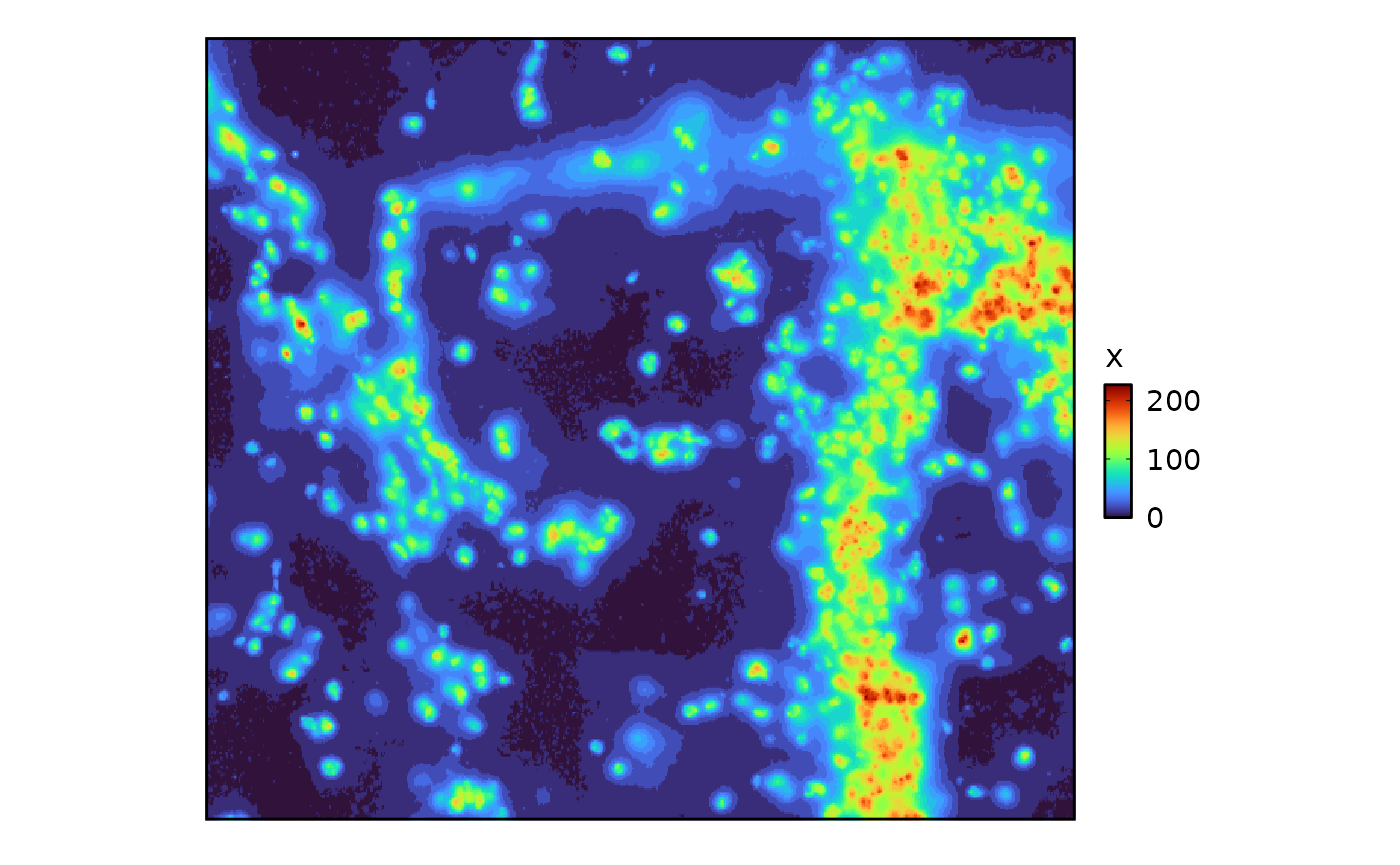

Masks are generally not plotted by scplotter, but can be plotted manually using plotthis::SpatMasksPlot()
Shapes are plotted using plotthis::SpatShapesPlot():

SpatShapesPlot(GiottoClass::getPolygonInfo(g))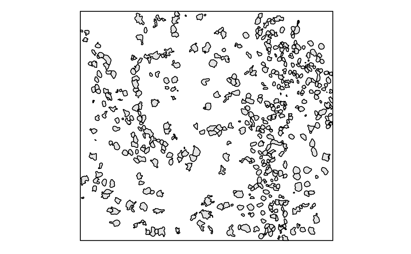

Points are plotted using plotthis::SpatPointsPlot():

SpatPointsPlot(GiottoClass::getSpatialLocations(g, output = "data.table"))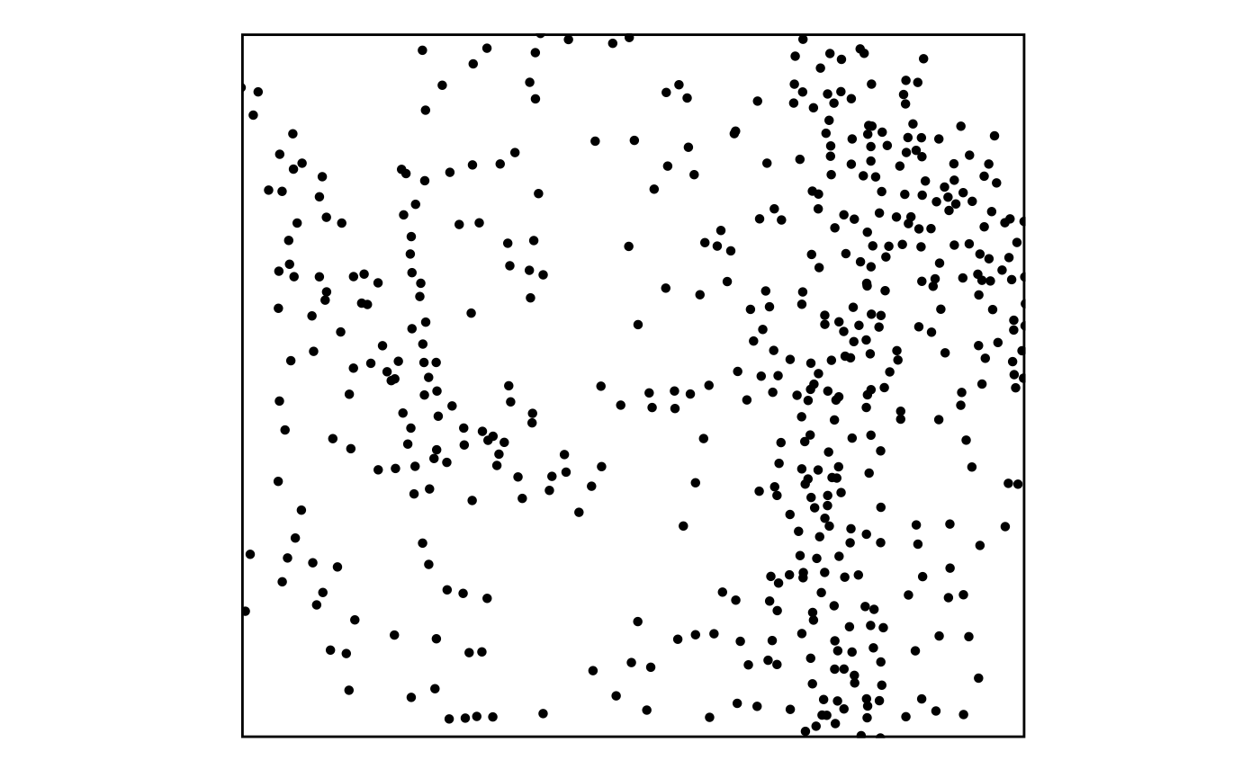

Flowchat of spatial data visualization

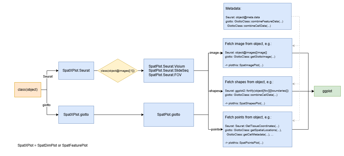
This diagram details the dispatch logic and internal structure of the SpatXPlot (SpatDimPlot or SpatFeaturePlot) function, which handles spatial visualizations for both Seurat and Giotto objects. The dispatch begins by checking class(object) and routes the call to either SpatXPlot.Seurat or SpatXPlot.giotto. In the Seurat case, if the image class (class(object@images[[1]])) is recognized (e.g., Visium, SlideSeq, FOV), it is further dispatched to a specialized SpatPlot.Seurat.<type> function.

Downstream, all implementations extract image, shapes, and points from the respective objects using methods like object@images[[image]], GetTissueCoordinates(...), or GiottoClass::getSpatialLocations(...). These are then passed to the unified plotting functions: SpatImagePlot, SpatShapesPlot, and SpatPointsPlot, before being assembled via ggplot. Additionally, the diagram notes access to metadata (e.g., object@meta.data or combineFeatureData(...)) that enhances these visualizations, by coloring points or shapes based on metadata attributes.

Controlling which layers to plot

To control which layers (image, shapes, points) are plotted in spatial visualization functions, you can use both specific arguments (image, shapes, points) and the general-purpose layers argument.

The layers argument is a character vector specifying which of “image”, “shapes”, “points” (and “masks”, if supported) to include, in the order they should be drawn. For example, layers = c("image", "points") will plot only the image and the points (if image and points are available in the object and they are enabled).

Individual logical flags like image, shapes, and points also let you enable or disable specific layers:

image = TRUE/FALSE enables/disables the image background; you can also provide an image name or color.

shapes = TRUE/FALSE controls whether shapes are plotted. It is automatically set to TRUE if shapes_fill_by is provided.

points = TRUE/FALSE defaults to TRUE, and controls whether spatial points (e.g., cells) are shown.

To fine-tune plotting further, use layer-specific argument prefixes such as image_, shapes_, points_ in the … to pass styling or data-specific options to the respective plotting functions (plotthis::SpatImagePlot(), etc.).

`SpatDimPlot` vs `SpatFeaturePlot`

The SpatDimPlot and SpatFeaturePlot functions are designed to visualize spatial data with different focuses:

SpatDimPlot: This function is used to visualize the data with categorical variables, borrowed from [Seurat::SpatialDimPlot][7]. The variables (specified by group_by) are applied to the points only.
SpatFeaturePlot: This function is used to visualize the data with continuous variables, borrowed from [Seurat::SpatialFeaturePlot][8]. The variables (specified by features) are applied to the points only.

Since the difference between these two functions is mainly on the points layer, so if you have points layer disabled, both functions will produce the same plot. The SpatDimPlot function is more suitable for categorical variables, while SpatFeaturePlot is more suitable for continuous variables.

When multiple features are provided with SpatFeaturePlot, the plots will be faceted. Each facet will show the spatial distribution of a single feature, allowing for a clear comparison across multiple features.

Visualizing the molecules

The molecules from the image based spatial data can be visualized using SpatDimPlot by specifying the group_by argument to "molecules" and provide the module list to the features argument. You can also use the nmols to limit the maximum number of each molecule to be plotted. This applies to both Seurat and giotto objects.

Visualizing in-situ vs non-in-situ points

It is hard to provide in-situ plots for Seurat objects by design. For giotto objects, the insitu points are only plotted necessary. For general purposes, for example, coloring the points by metadata, non-in-situ points are plotted by default. But when one requires use_overlap = TRUE (see also: https://drieslab.github.io/GiottoVisuals/reference/spatInSituPlotPoints.html#arg-use-overlap), the in-situ points are plotted.