
Visualizes single-cell data in reduced dimension space (e.g., UMAP, t-SNE, PCA). This is the primary function for exploring cell clustering, cell identity, and spatial relationships in transcriptomics datasets. It creates scatter plots where each point represents a cell, positioned by its coordinates in the reduced dimension space and colored by metadata variables such as cell type, sample condition, or cluster assignment.
CellDimPlot serves as a unified interface across multiple single-cell data
containers:
Seurat objects — Extracts embeddings from
Reductions()and metadata from@meta.data. The default reduction is auto-detected viadefault_dimreduc().Giotto objects — Extracts spatial dimension reductions and cell metadata using
spat_unitandfeat_typeto identify the correct spatial unit and feature type.h5ad files (.h5ad or opened
H5File) — Reads fromobsmfor embeddings andobsfor metadata. Reduction names are automatically prefixed with"X_"when needed (e.g.,"umap"→"X_umap").
Beyond basic cluster visualization, CellDimPlot supports a rich set of
visual overlays and analytical enhancements:
Cluster highlighting — Emphasize cells matching a logical expression while dimming others (
highlight).Group labels — Add text labels at group centroids (
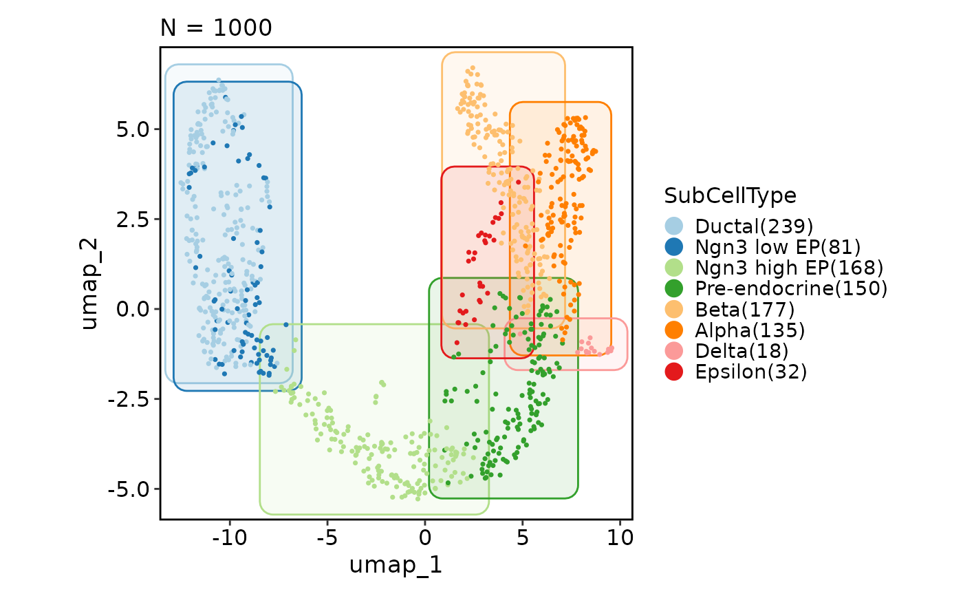
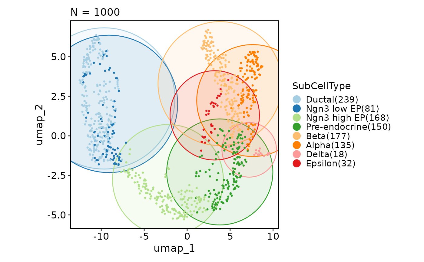
label,label_insitu).Group marks — Draw boundary shapes around groups: ellipse, rectangle, or circle (
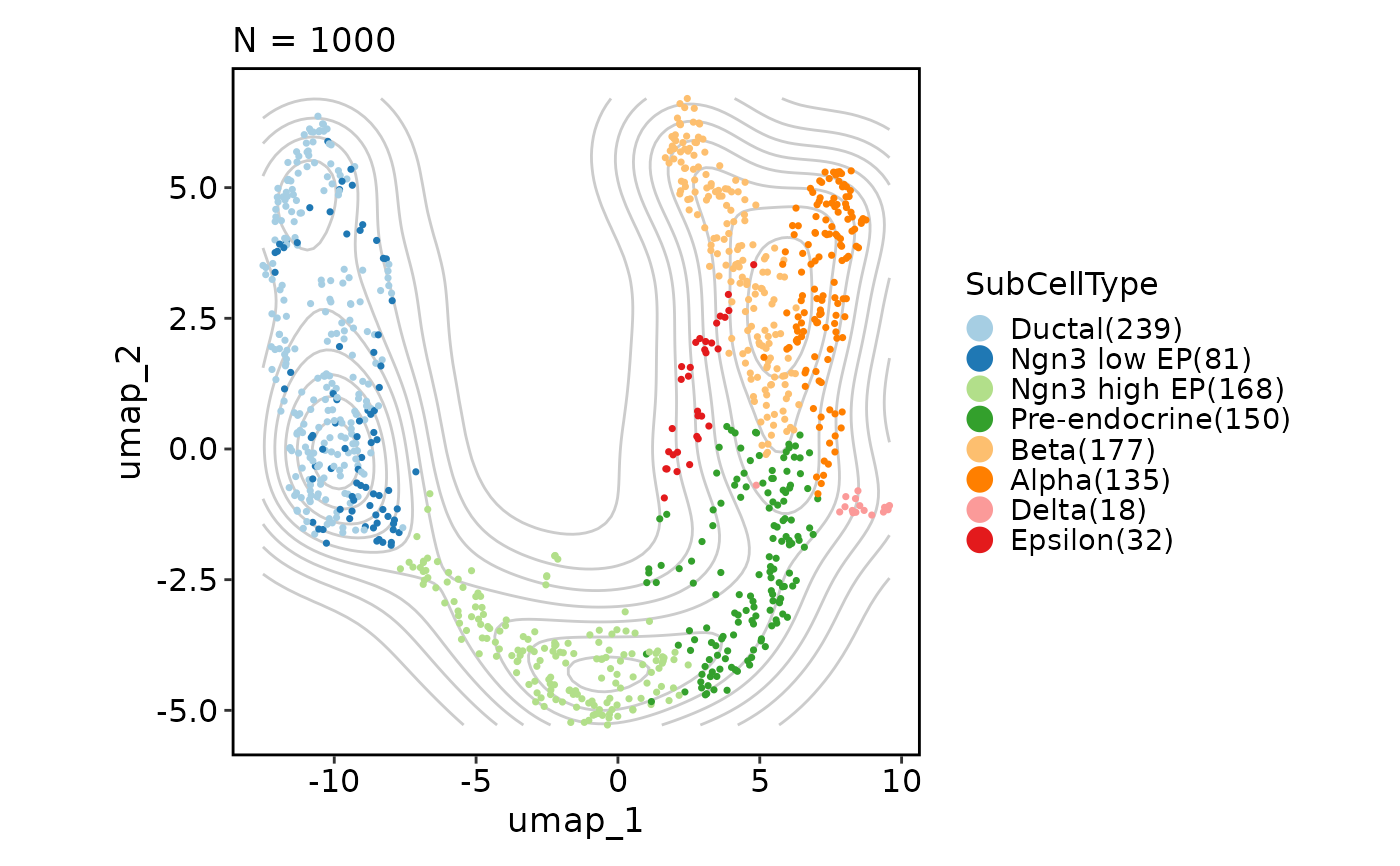
add_mark,mark_type).Density contours — Overlay 2D density estimates (
add_density).Neighbor graphs — Draw edges between neighboring cells from k-NN or shared-nearest-neighbor graphs (
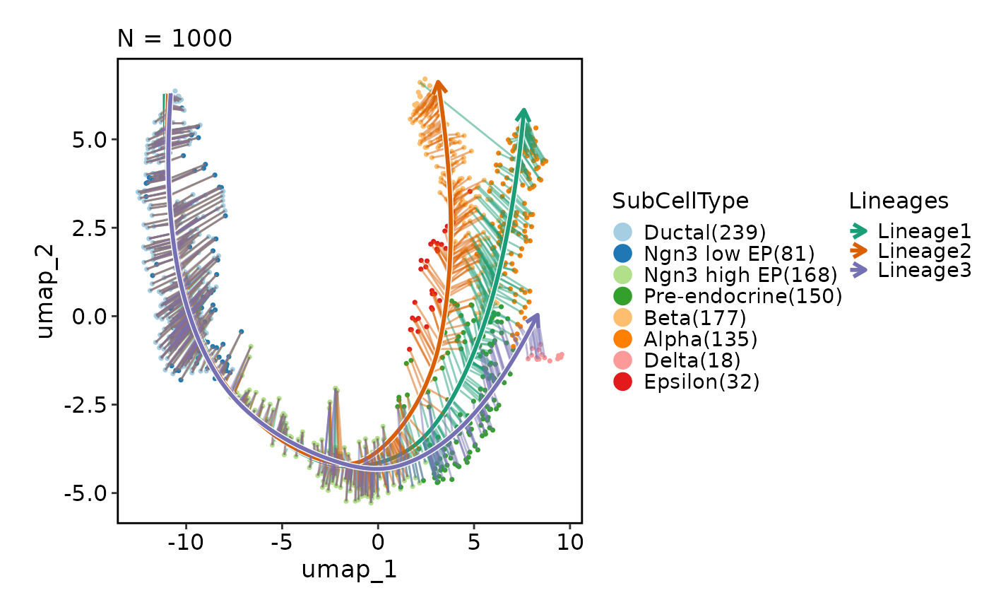
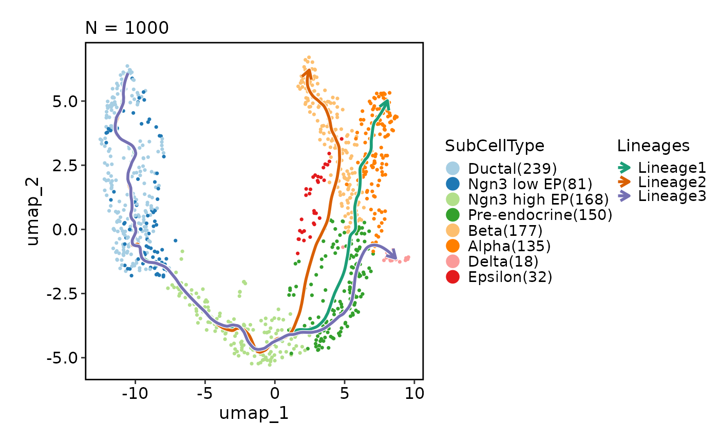
graph).Lineage trajectories — Overlay pseudotime lineage curves (
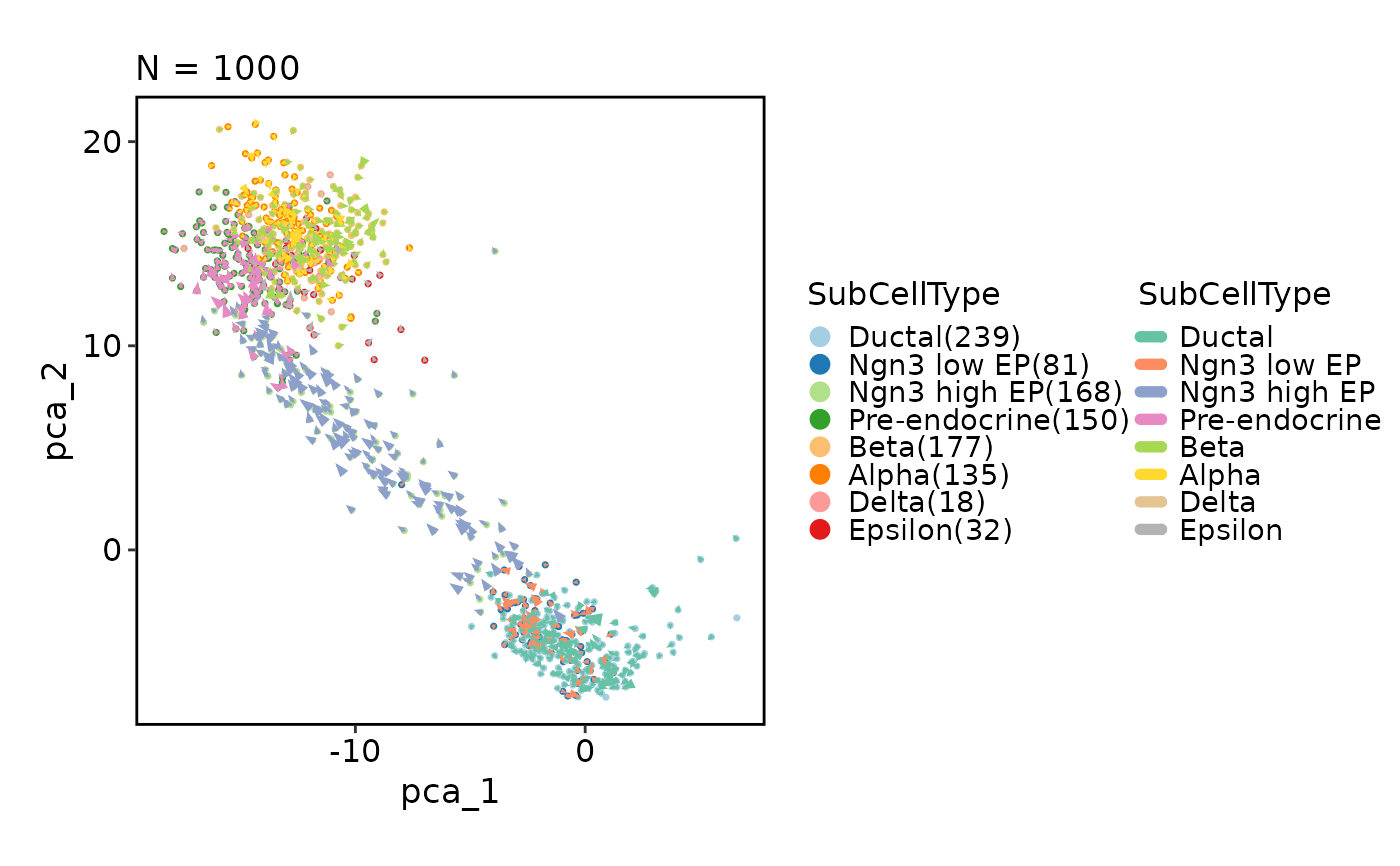
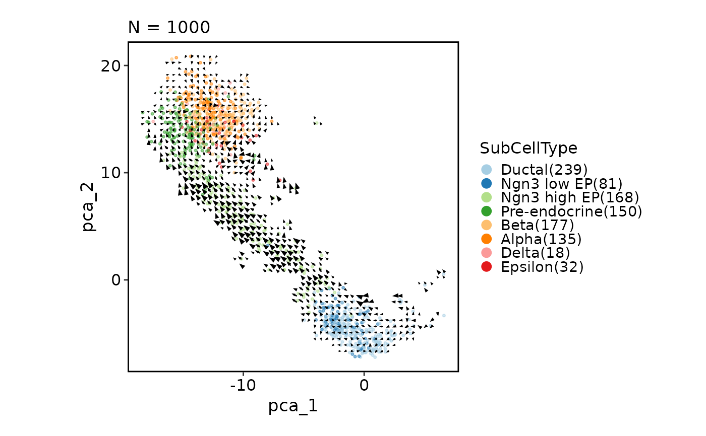
lineages).Velocity arrows — Overlay RNA velocity vectors on the embedding (
velocity). For dedicated velocity visualization with grid or stream plots, seeCellVelocityPlot.Statistical charts — Embed small bar, ring, or line charts at group positions showing composition of a second variable (
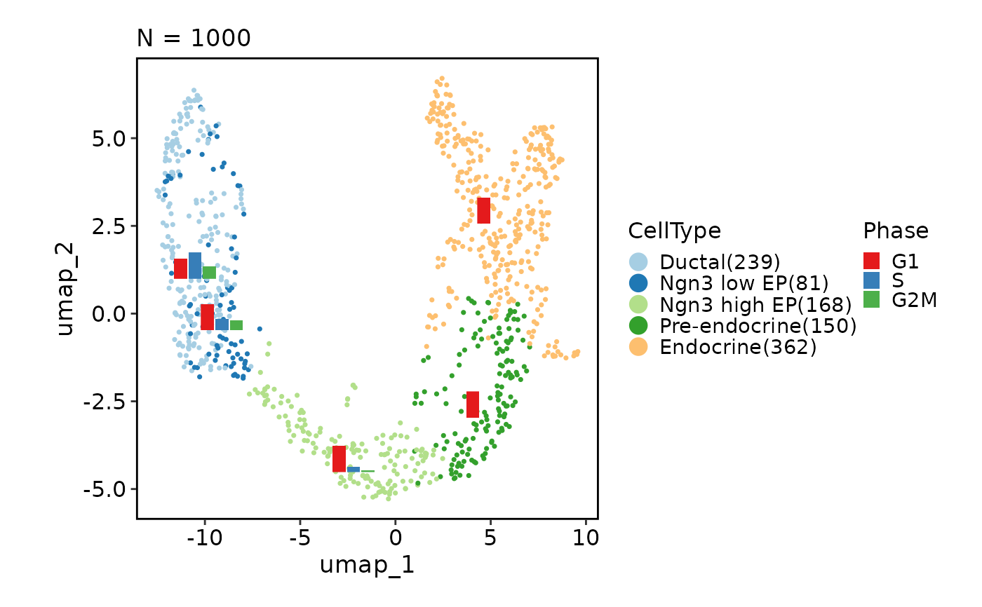
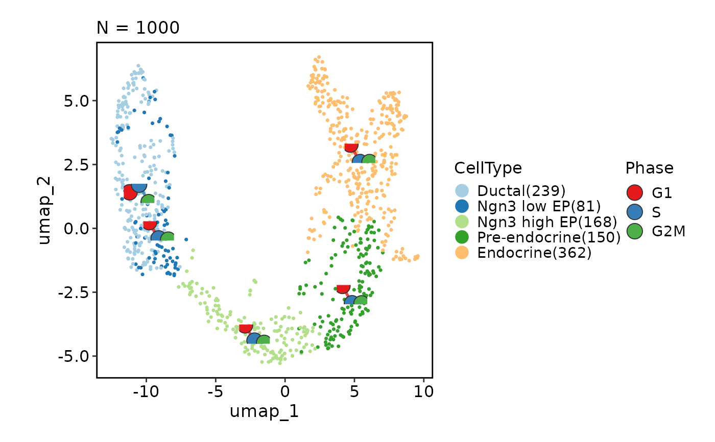
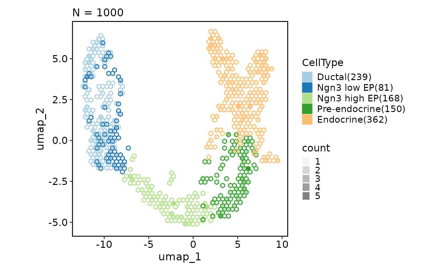
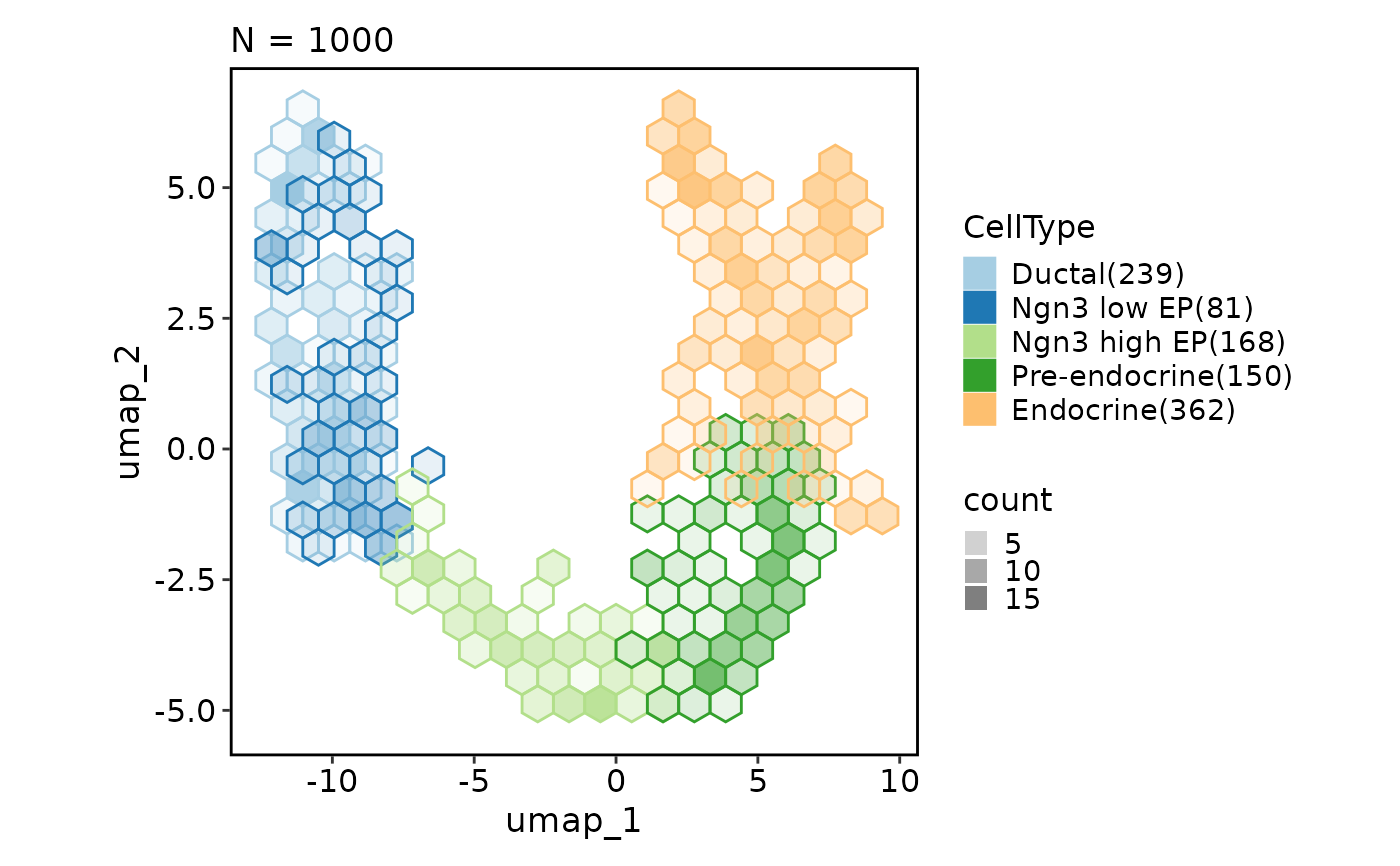
stat_by,stat_plot_type).Hexagonal binning — Replace scatter points with binned hexagons for large datasets (
hex).3D visualization — Plot three dimensions by specifying
dims = 1:3.Rasterization — Render points as a raster image for performance with large cell counts (
raster).
Usage
CellDimPlot(
  object,
  reduction = NULL,
  graph = NULL,
  group_by = NULL,
  ident = NULL,
  spat_unit = NULL,
  feat_type = NULL,
  velocity = NULL,
  ...
)
Arguments
- object
A Seurat object, a Giotto object, a path to an
.h5adfile, or an openedH5Filefrom the hdf5r package.- reduction
Name of the dimension reduction to plot. Typical values are
"umap","tsne", or"pca". For Seurat objects, the default reduction is auto-detected viadefault_dimreduc(). For h5ad files, the prefix"X_"is added automatically when needed (i.e.,"umap"is treated as"X_umap"if"umap"alone is not found). For Giotto objects, this parameter is required unless a default reduction has been set.- graph
Name of the neighbor graph used to draw edges between neighboring cells on the plot. For Seurat objects, this is a graph name in
Graphs(object)(e.g.,"RNA_nn","RNA_snn"). For Giotto objects, this is a nearest-neighbor network name; setgraph = TRUEto use the first available network. For h5ad files, connectivities are read fromobsp[["connectivities"]]. SettinggraphtoNULL(the default) suppresses edge drawing.- group_by
Character vector of metadata column name(s) used to color the cells. Can be a single column (e.g.,
"CellType") or multiple columns for combined grouping. Default isNULL, which falls back to the active identity for Seurat objects and is required for other object types.- ident
Alias for
group_by, provided for compatibility with Seurat's naming convention. When bothgroup_byandidentare specified, they must be identical.- spat_unit
Spatial unit name for Giotto objects (e.g.,
"cell"). Ignored for Seurat and h5ad inputs. IfNULL, the default spatial unit is auto-detected viaGiottoClass::set_default_spat_unit().- feat_type
Feature type name for Giotto objects (e.g.,
"rna","dna","protein"). Ignored for Seurat and h5ad inputs. IfNULL, the default feature type is auto-detected viaGiottoClass::set_default_feat_type().- velocity
Name of a velocity reduction whose first two dimensions encode RNA velocity vectors to overlay on the plot. Typical values are
"stochastic_<reduction>","deterministic_<reduction>", or"dynamical_<reduction>"(e.g.,"stochastic_UMAP"). For dedicated velocity visualization (grid or stream plots), useCellVelocityPlotinstead. Default isNULL(no velocity overlay).- ...
Additional arguments passed to
plotthis::DimPlot(). Key parameters include:Appearance:
pt_size,pt_alpha,palette,palcolor,theme,theme_args,legend.position,legend.directionHighlighting:
highlight— a logical expression as a string (e.g.,'CellType == "Beta"') to emphasize matching cellsLabels:
label,label_insitu,label_repel,label_fg,label_bg,label_size,label_segment_colorGroup marks:
add_mark,mark_type("ellipse","rect","circle"),mark_expand,mark_alpha,mark_linetypeDensity:
add_density,density_filled,density_filled_paletteLineages:
lineages,lineages_whiskers,lineages_spanStatistical charts:
stat_by,stat_plot_type("ring","bar","line"),stat_type("percent","count"),stat_plot_label,stat_plot_size,stat_argsHexagonal binning:
hex,hex_bins,hex_countRendering:
raster,raster_dpiDimensionality:
dims— which dimensions to plot (default1:2; set to1:3for 3D)Layout:
split_by,facet_by,combine,nrow,ncol
Details
See the following vignettes for examples with Giotto objects:
https://pwwang.github.io/scplotter/articles/Giotto_CODEX.html
https://pwwang.github.io/scplotter/articles/Giotto_seqFISH.html
https://pwwang.github.io/scplotter/articles/Giotto_SlideSeq.html
https://pwwang.github.io/scplotter/articles/Giotto_Spatial_CITE-Seq.html
https://pwwang.github.io/scplotter/articles/Giotto_Visium.html
https://pwwang.github.io/scplotter/articles/Giotto_VisiumHD.html
https://pwwang.github.io/scplotter/articles/Giotto_Xenium.html
And for examples with h5ad files:
Note
Default reduction for Seurat objects: When reduction = NULL,
CellDimPlot calls default_dimreduc(object) to determine the default
reduction. For Seurat >= 5.4.0, this uses the official
DefaultDimReduc getter; for older versions, it falls back to
object@misc$DefaultDimReduc.
Giotto spatial units and feature types: The spat_unit and feat_type
parameters are required to locate the correct data within Giotto's
hierarchical spatial data structure. When NULL, Giotto's own default
resolution is used, which is typically sufficient for standard analyses.
Performance with large datasets: For datasets with many cells (e.g.,
over 50,000), consider using raster = TRUE to render points as a raster
image, or hex = TRUE to use hexagonal binning. Both options significantly
reduce rendering time and output file size.
Factor ordering: The order of groups in the legend follows the factor
levels of the group_by column. Set factor levels on your metadata column
before plotting to control legend order.
Data extraction
The function extracts cell embeddings and metadata from the input object,
combines them into a single data frame, and passes the result to
plotthis::DimPlot() along with any additional
arguments provided via .... The extraction logic varies by object type:
Seurat objects: Embeddings(object, reduction) provides the coordinates;
object@meta.data provides the metadata. When group_by is NULL,
Idents(object) is used as the default grouping variable (column name
"Identity"). The graph parameter references object@graphs.
Giotto objects: getDimReduction() with output = "matrix" provides
coordinates; getCellMetadata() with output = "data.table" provides
metadata. Both spat_unit and feat_type are resolved to defaults if not
specified. The graph parameter references nearest-neighbor networks
retrieved via getNearestNetwork() and converted with igraph.
h5ad files: obsm[[reduction]] provides the embedding matrix;
obs provides metadata (decoded via h5group_to_dataframe() for
categorical variables). The graph parameter references
obsp[["connectivities"]], converted via igraph to an adjacency
matrix.
Velocity overlay
When velocity is specified, velocity vectors are overlaid on the dimension
reduction plot. The velocity parameter names a second reduction
(e.g., "stochastic_UMAP") whose first two dimensions encode the velocity
arrows. This is a lightweight overlay — for dedicated velocity visualization
with grid or stream plots, use CellVelocityPlot which delegates to
plotthis::VelocityPlot().
See also
plotthis::DimPlot()— The underlying plotting engineCellVelocityPlot— Dedicated RNA velocity visualizationCellStatPlot— Statistical summaries and comparisons
Examples
# \donttest{
set.seed(8525)
data(pancreas_sub)
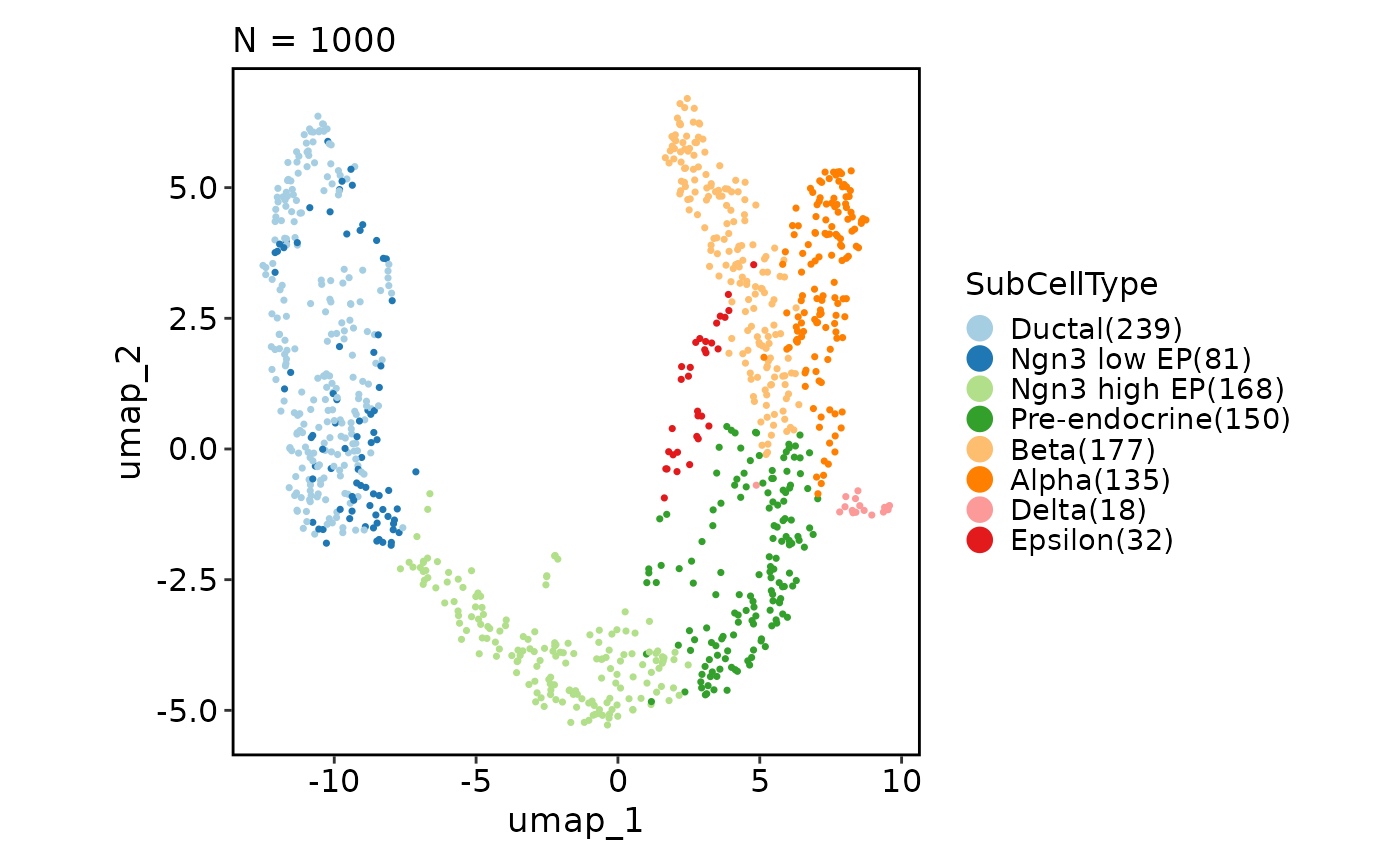
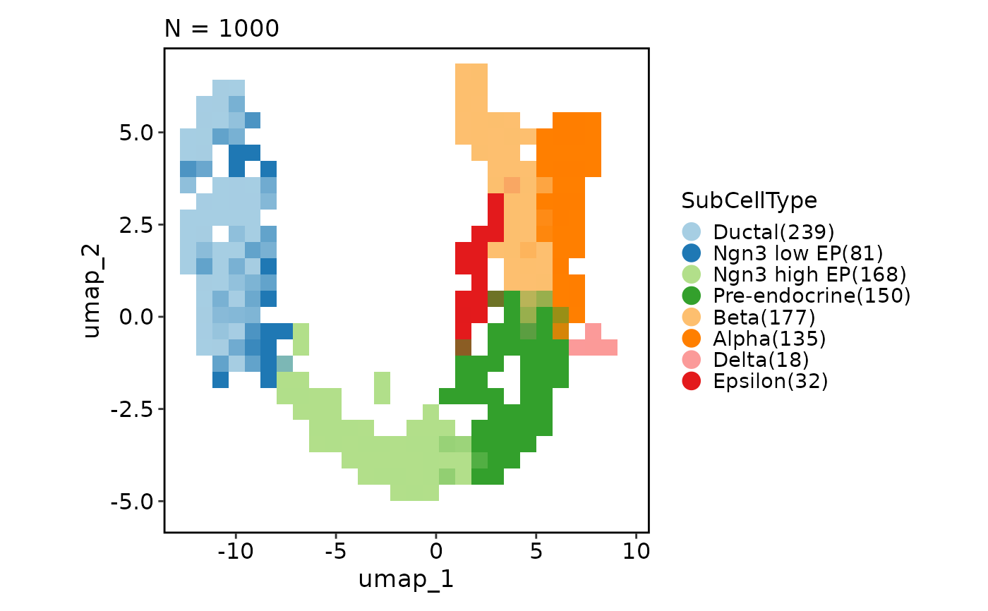
CellDimPlot(pancreas_sub, group_by = "SubCellType", reduction = "UMAP")
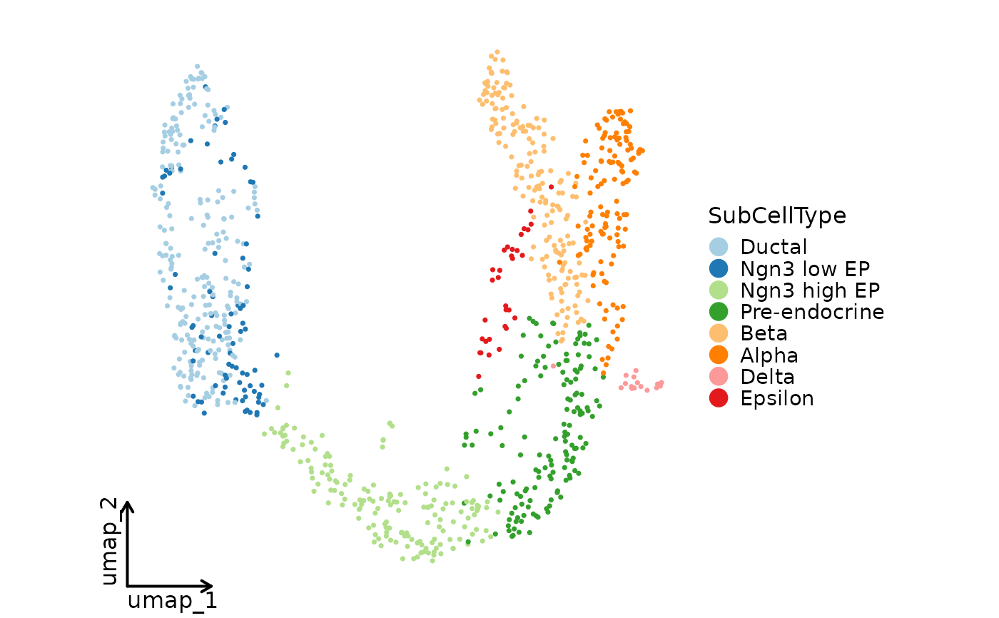
 CellDimPlot(pancreas_sub, group_by = "SubCellType", reduction = "UMAP",
theme = "theme_blank")
CellDimPlot(pancreas_sub, group_by = "SubCellType", reduction = "UMAP",
theme = "theme_blank")
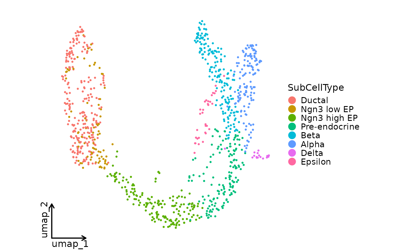
 CellDimPlot(pancreas_sub, group_by = "SubCellType", reduction = "UMAP",
palette = "seurat", theme = "theme_blank")
CellDimPlot(pancreas_sub, group_by = "SubCellType", reduction = "UMAP",
palette = "seurat", theme = "theme_blank")
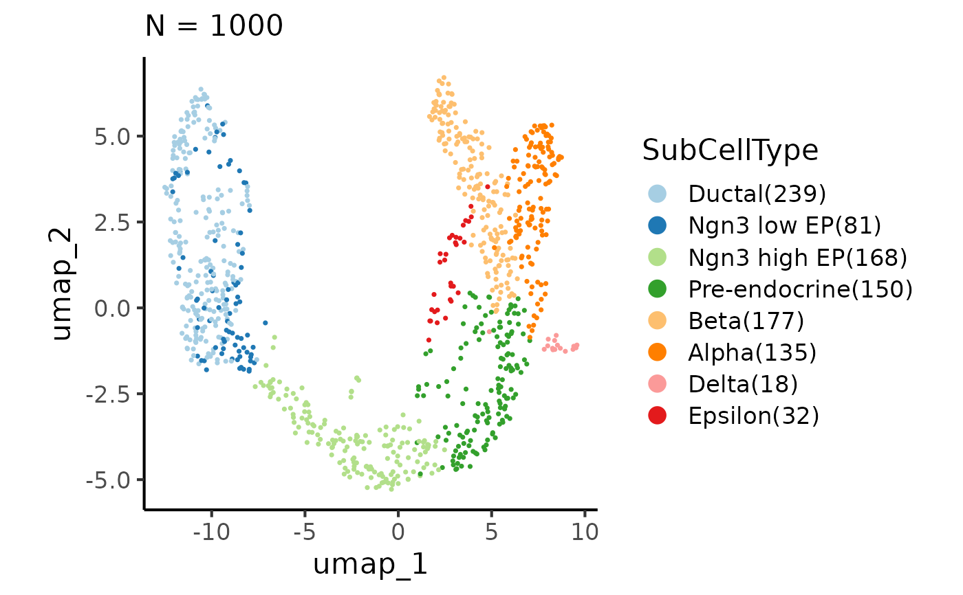
 CellDimPlot(pancreas_sub, group_by = "SubCellType", reduction = "UMAP",
theme = ggplot2::theme_classic, theme_args = list(base_size = 16))
CellDimPlot(pancreas_sub, group_by = "SubCellType", reduction = "UMAP",
theme = ggplot2::theme_classic, theme_args = list(base_size = 16))
 CellDimPlot(pancreas_sub, group_by = "SubCellType", reduction = "UMAP",
raster = TRUE, raster_dpi = 30)
CellDimPlot(pancreas_sub, group_by = "SubCellType", reduction = "UMAP",
raster = TRUE, raster_dpi = 30)
 # Highlight cells
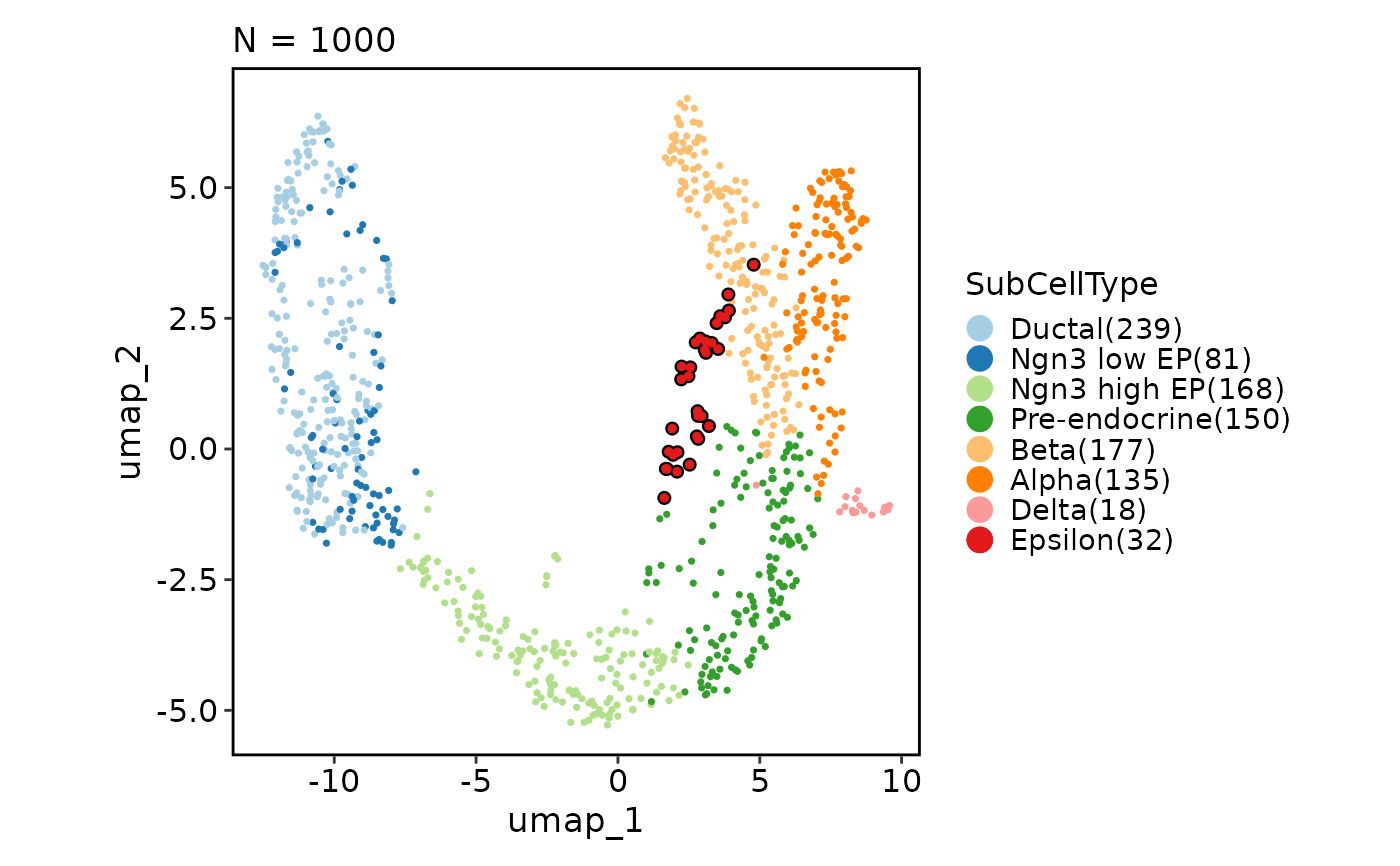
CellDimPlot(pancreas_sub,
group_by = "SubCellType", reduction = "UMAP",
highlight = 'SubCellType == "Epsilon"'
)
# Highlight cells
CellDimPlot(pancreas_sub,
group_by = "SubCellType", reduction = "UMAP",
highlight = 'SubCellType == "Epsilon"'
)
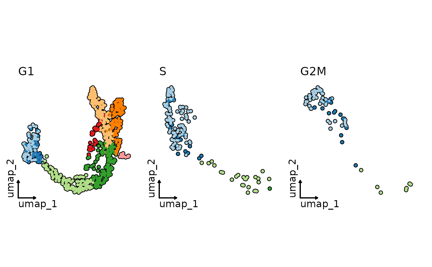
 CellDimPlot(pancreas_sub,
group_by = "SubCellType", split_by = "Phase", reduction = "UMAP",
highlight = TRUE, theme = "theme_blank", legend.position = "none"
)
CellDimPlot(pancreas_sub,
group_by = "SubCellType", split_by = "Phase", reduction = "UMAP",
highlight = TRUE, theme = "theme_blank", legend.position = "none"
)
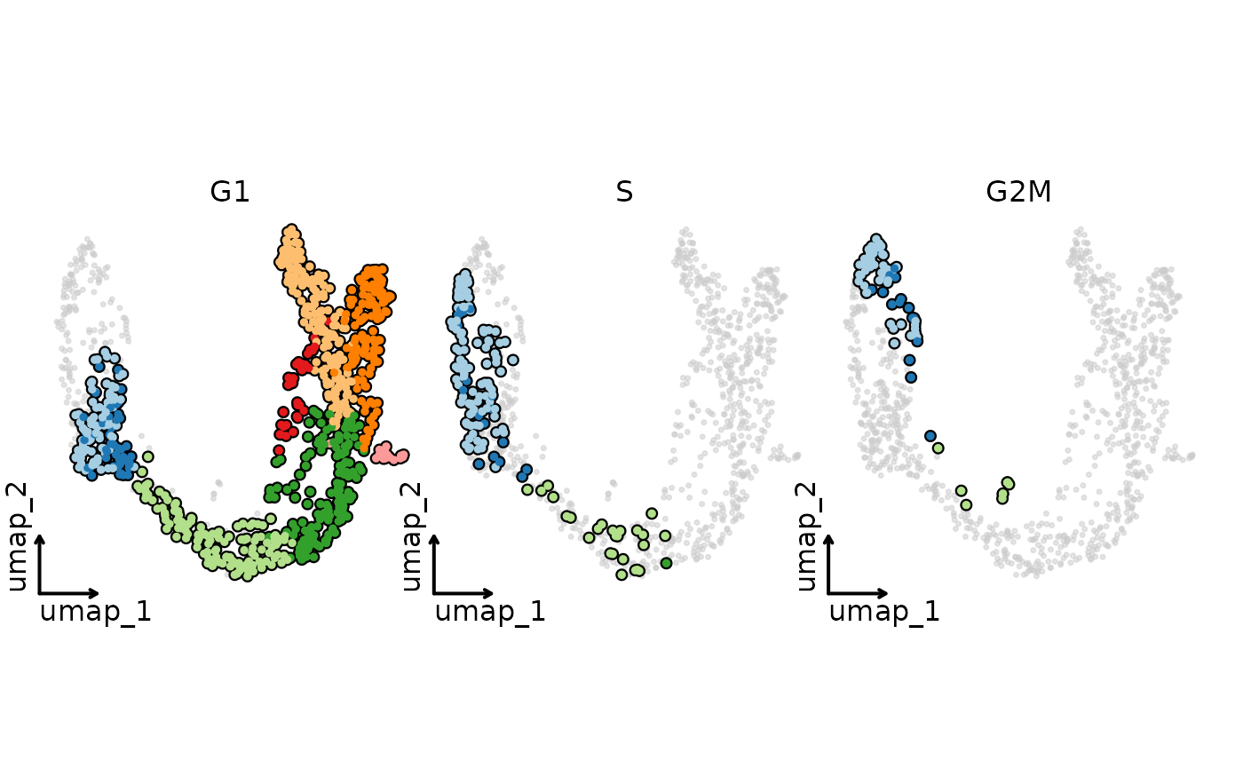
 CellDimPlot(pancreas_sub,
group_by = "SubCellType", facet_by = "Phase", reduction = "UMAP",
highlight = TRUE, theme = "theme_blank", legend.position = "none"
)
CellDimPlot(pancreas_sub,
group_by = "SubCellType", facet_by = "Phase", reduction = "UMAP",
highlight = TRUE, theme = "theme_blank", legend.position = "none"
)
 # Add group labels
CellDimPlot(pancreas_sub, group_by = "SubCellType", reduction = "UMAP",
label = TRUE)
# Add group labels
CellDimPlot(pancreas_sub, group_by = "SubCellType", reduction = "UMAP",
label = TRUE)
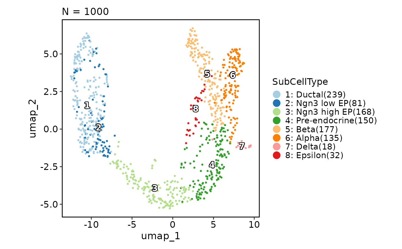 CellDimPlot(pancreas_sub,
group_by = "SubCellType", reduction = "UMAP",
label = TRUE, label_fg = "orange", label_bg = "red", label_size = 5
)
CellDimPlot(pancreas_sub,
group_by = "SubCellType", reduction = "UMAP",
label = TRUE, label_fg = "orange", label_bg = "red", label_size = 5
)
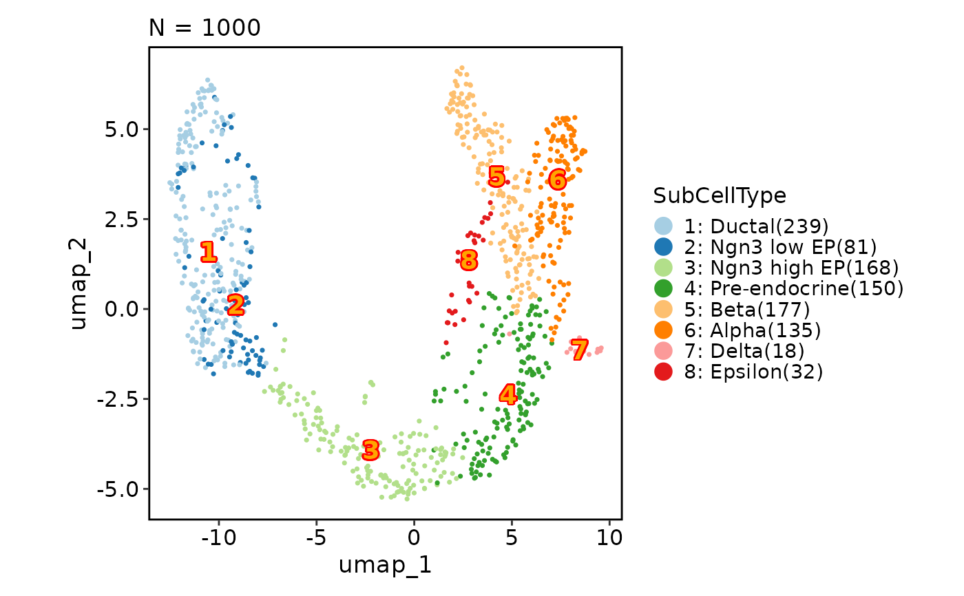 CellDimPlot(pancreas_sub,
group_by = "SubCellType", reduction = "UMAP",
label = TRUE, label_insitu = TRUE
)
CellDimPlot(pancreas_sub,
group_by = "SubCellType", reduction = "UMAP",
label = TRUE, label_insitu = TRUE
)
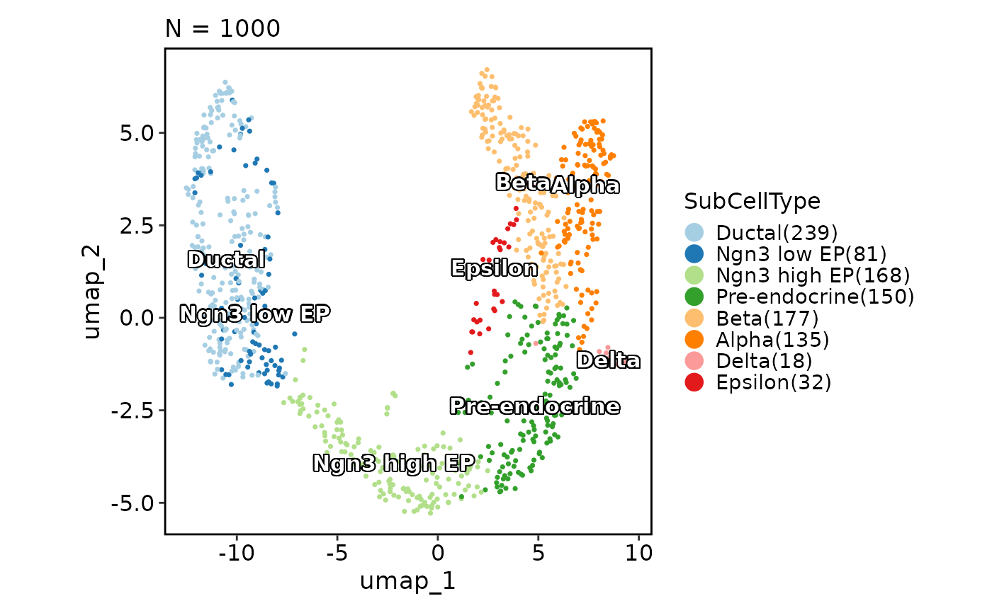 CellDimPlot(pancreas_sub,
group_by = "SubCellType", reduction = "UMAP",
label = TRUE, label_insitu = TRUE, label_repel = TRUE,
label_segment_color = "red"
)
CellDimPlot(pancreas_sub,
group_by = "SubCellType", reduction = "UMAP",
label = TRUE, label_insitu = TRUE, label_repel = TRUE,
label_segment_color = "red"
)
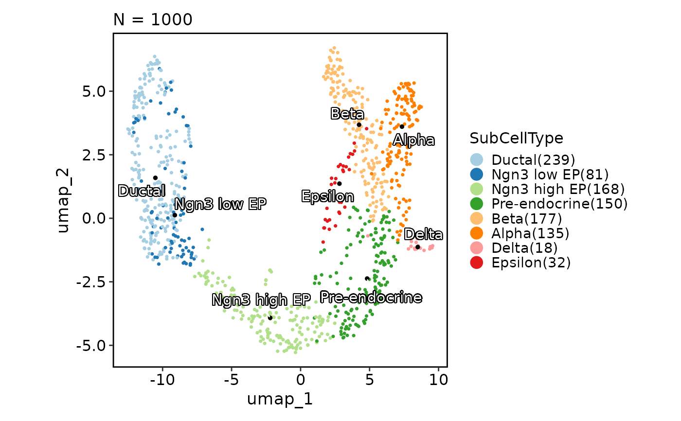 # Add various shape of marks
CellDimPlot(pancreas_sub, group_by = "SubCellType", reduction = "UMAP",
add_mark = TRUE)
# Add various shape of marks
CellDimPlot(pancreas_sub, group_by = "SubCellType", reduction = "UMAP",
add_mark = TRUE)
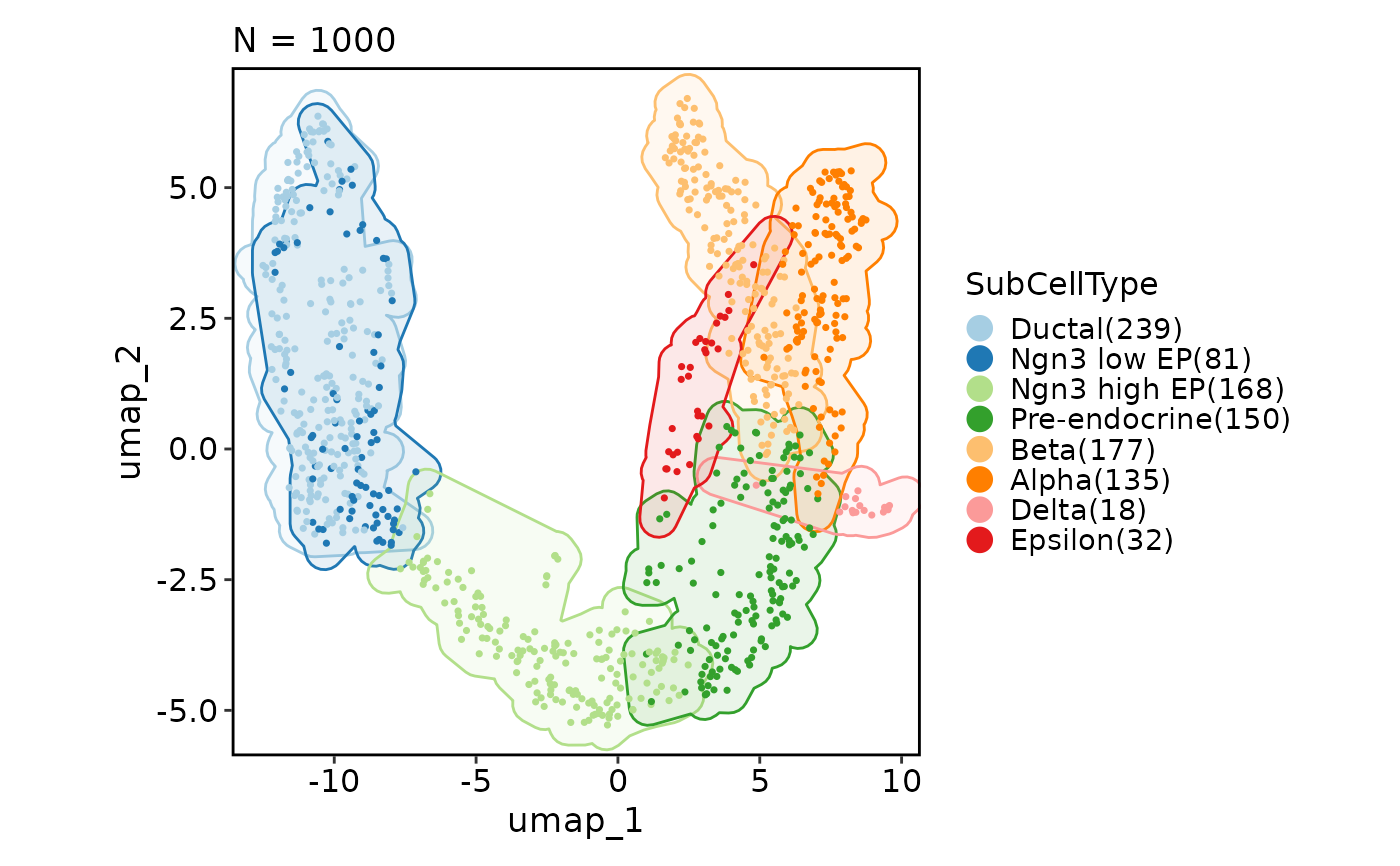 CellDimPlot(pancreas_sub, group_by = "SubCellType", reduction = "UMAP",
add_mark = TRUE, mark_expand = grid::unit(1, "mm"))
CellDimPlot(pancreas_sub, group_by = "SubCellType", reduction = "UMAP",
add_mark = TRUE, mark_expand = grid::unit(1, "mm"))
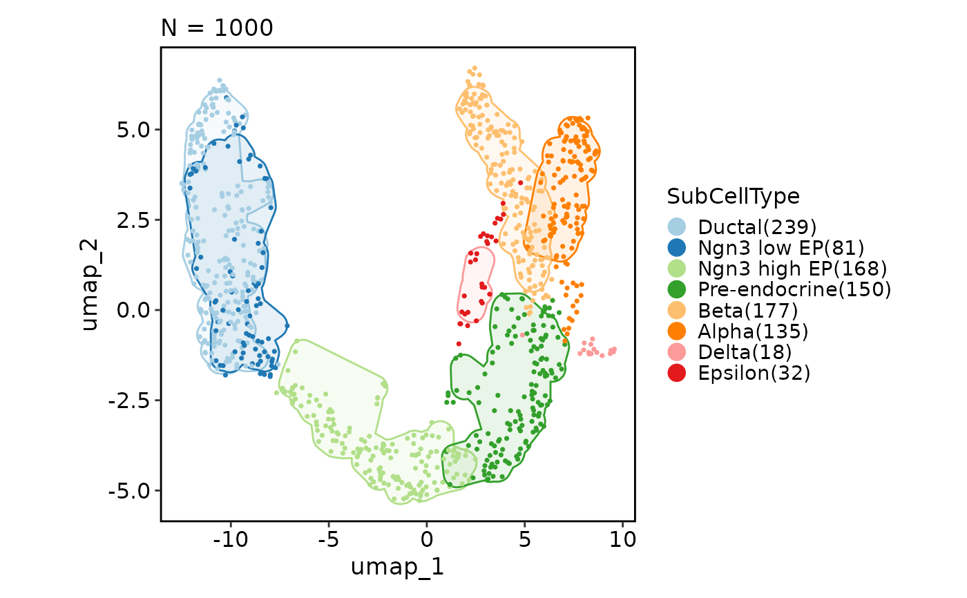 CellDimPlot(pancreas_sub, group_by = "SubCellType", reduction = "UMAP",
add_mark = TRUE, mark_alpha = 0.3)
CellDimPlot(pancreas_sub, group_by = "SubCellType", reduction = "UMAP",
add_mark = TRUE, mark_alpha = 0.3)
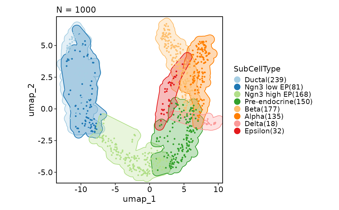 CellDimPlot(pancreas_sub, group_by = "SubCellType", reduction = "UMAP",
add_mark = TRUE, mark_linetype = 2)
CellDimPlot(pancreas_sub, group_by = "SubCellType", reduction = "UMAP",
add_mark = TRUE, mark_linetype = 2)
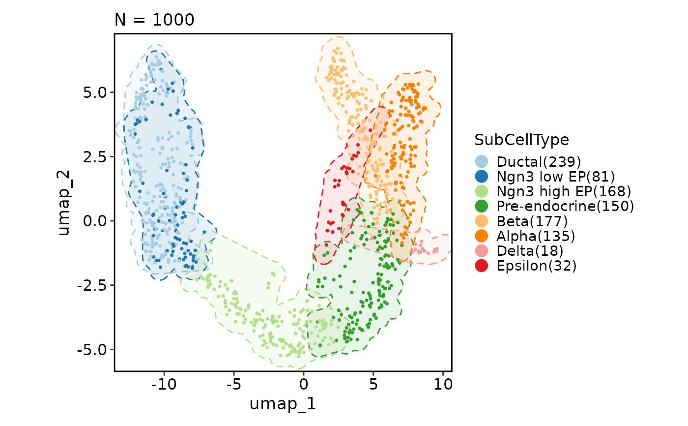 CellDimPlot(pancreas_sub, group_by = "SubCellType", reduction = "UMAP",
add_mark = TRUE, mark_type = "ellipse")
CellDimPlot(pancreas_sub, group_by = "SubCellType", reduction = "UMAP",
add_mark = TRUE, mark_type = "ellipse")
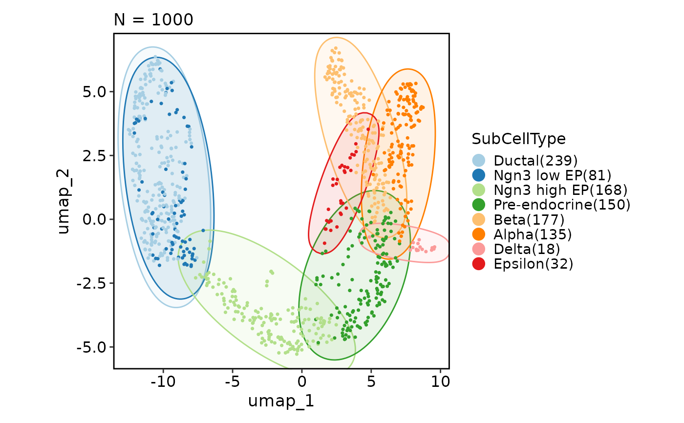 CellDimPlot(pancreas_sub, group_by = "SubCellType", reduction = "UMAP",
add_mark = TRUE, mark_type = "rect")
CellDimPlot(pancreas_sub, group_by = "SubCellType", reduction = "UMAP",
add_mark = TRUE, mark_type = "rect")
 CellDimPlot(pancreas_sub, group_by = "SubCellType", reduction = "UMAP",
add_mark = TRUE, mark_type = "circle")
CellDimPlot(pancreas_sub, group_by = "SubCellType", reduction = "UMAP",
add_mark = TRUE, mark_type = "circle")
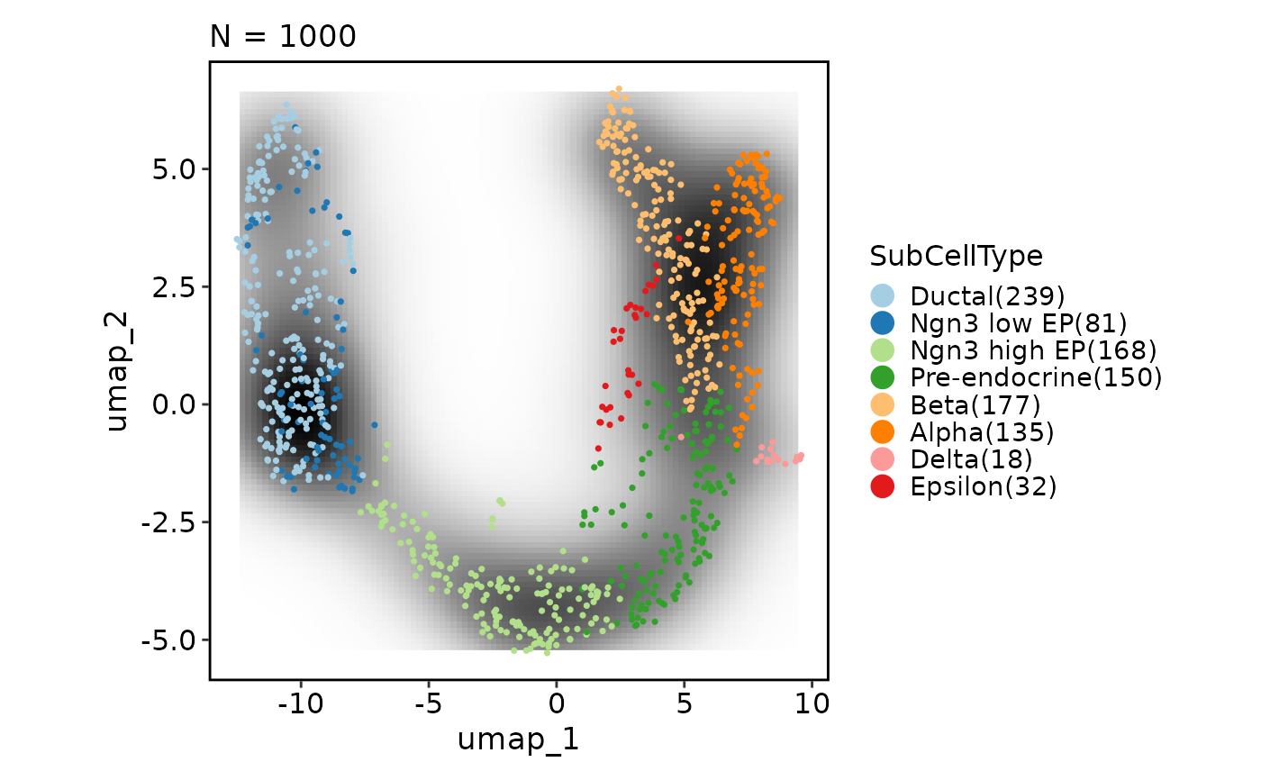
 # Add a density layer
CellDimPlot(pancreas_sub, group_by = "SubCellType", reduction = "UMAP",
add_density = TRUE)
# Add a density layer
CellDimPlot(pancreas_sub, group_by = "SubCellType", reduction = "UMAP",
add_density = TRUE)
 CellDimPlot(pancreas_sub, group_by = "SubCellType", reduction = "UMAP",
add_density = TRUE, density_filled = TRUE)
#> Warning: Removed 396 rows containing missing values or values outside the scale range
#> (`geom_raster()`).
CellDimPlot(pancreas_sub, group_by = "SubCellType", reduction = "UMAP",
add_density = TRUE, density_filled = TRUE)
#> Warning: Removed 396 rows containing missing values or values outside the scale range
#> (`geom_raster()`).
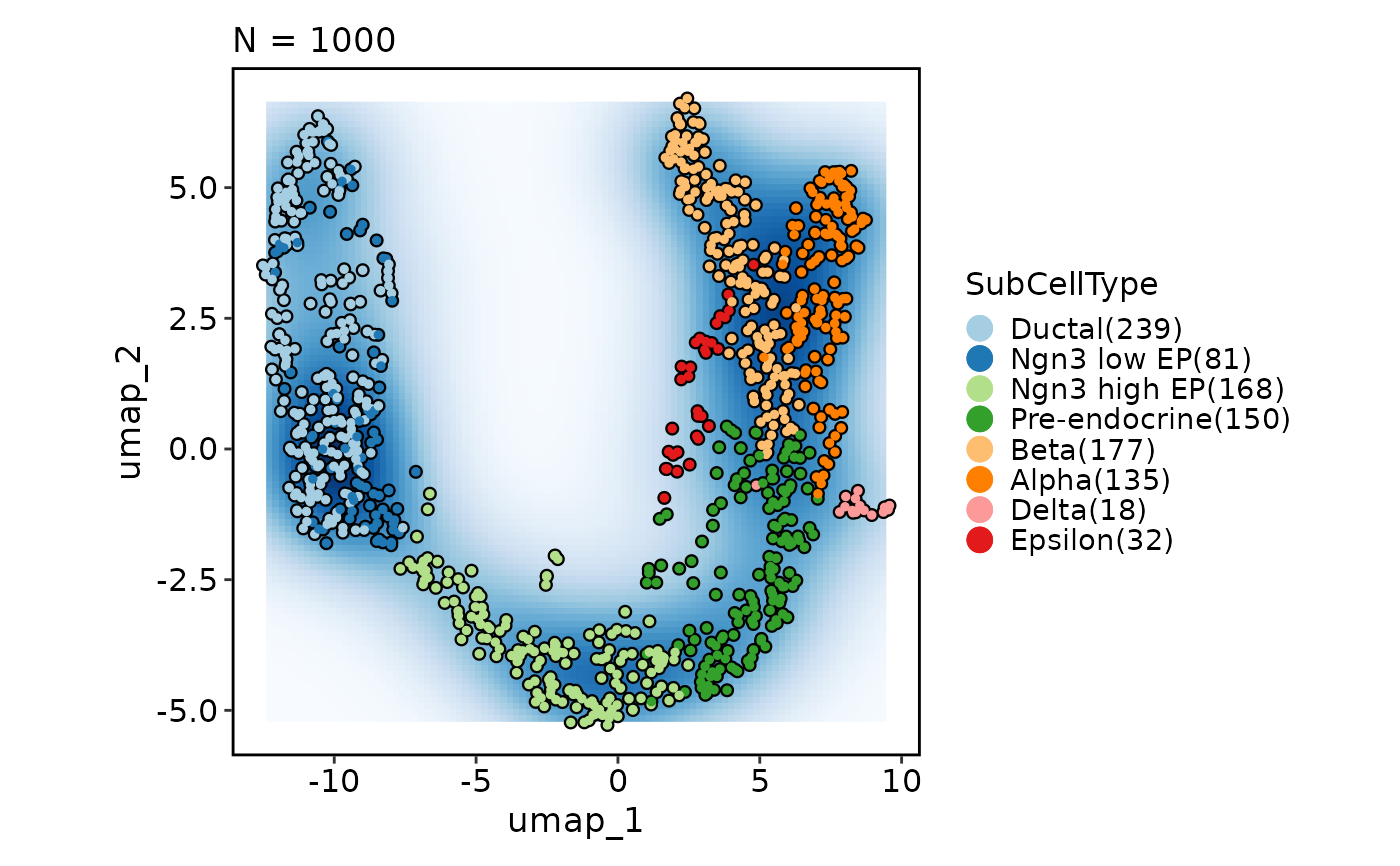
 CellDimPlot(pancreas_sub,
group_by = "SubCellType", reduction = "UMAP",
add_density = TRUE, density_filled = TRUE, density_filled_palette = "Blues",
highlight = TRUE
)
#> Warning: Removed 396 rows containing missing values or values outside the scale range
#> (`geom_raster()`).
CellDimPlot(pancreas_sub,
group_by = "SubCellType", reduction = "UMAP",
add_density = TRUE, density_filled = TRUE, density_filled_palette = "Blues",
highlight = TRUE
)
#> Warning: Removed 396 rows containing missing values or values outside the scale range
#> (`geom_raster()`).
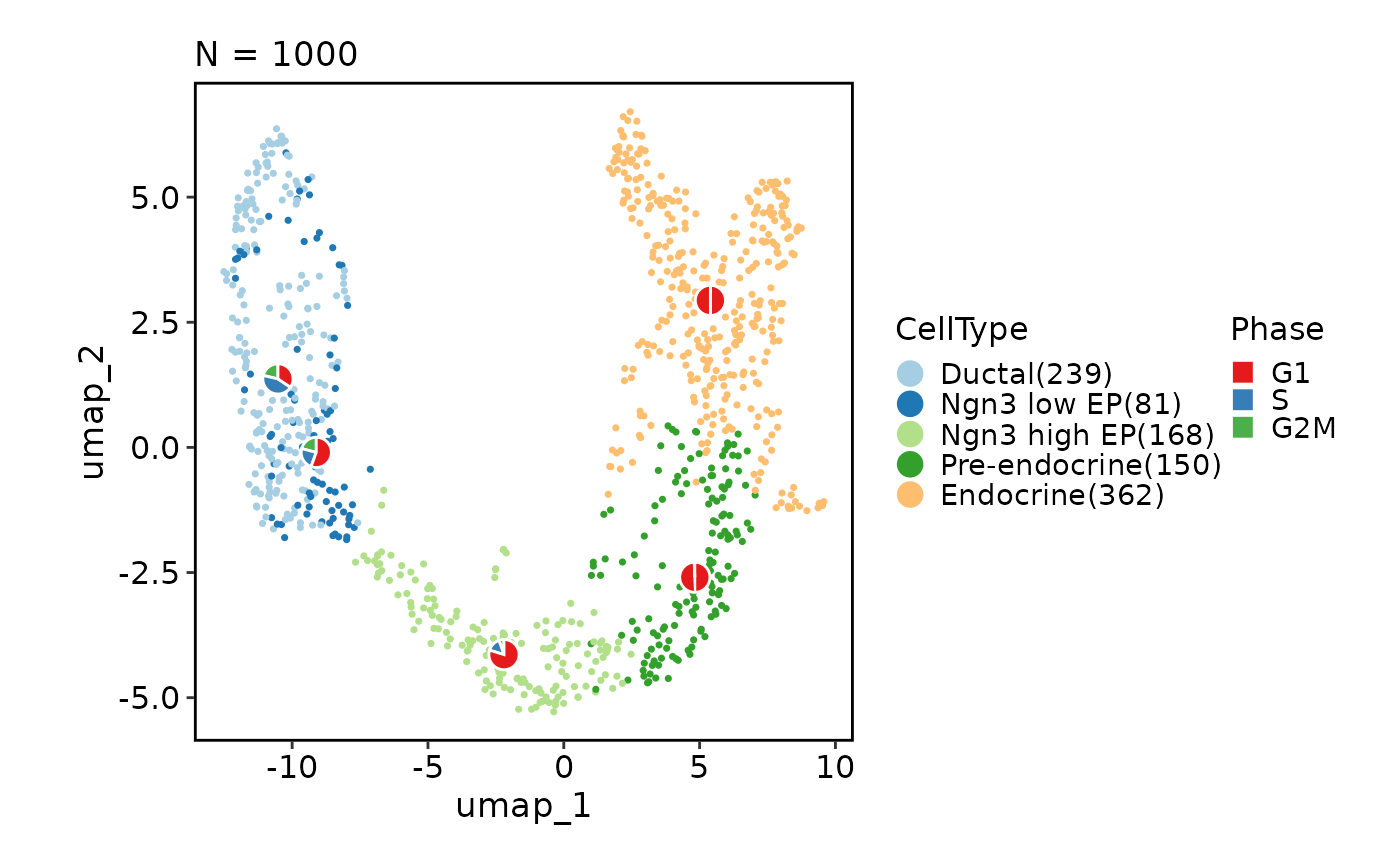
 # Add statistical charts
CellDimPlot(pancreas_sub,
group_by = "CellType", reduction = "UMAP", stat_by = "Phase")
# Add statistical charts
CellDimPlot(pancreas_sub,
group_by = "CellType", reduction = "UMAP", stat_by = "Phase")
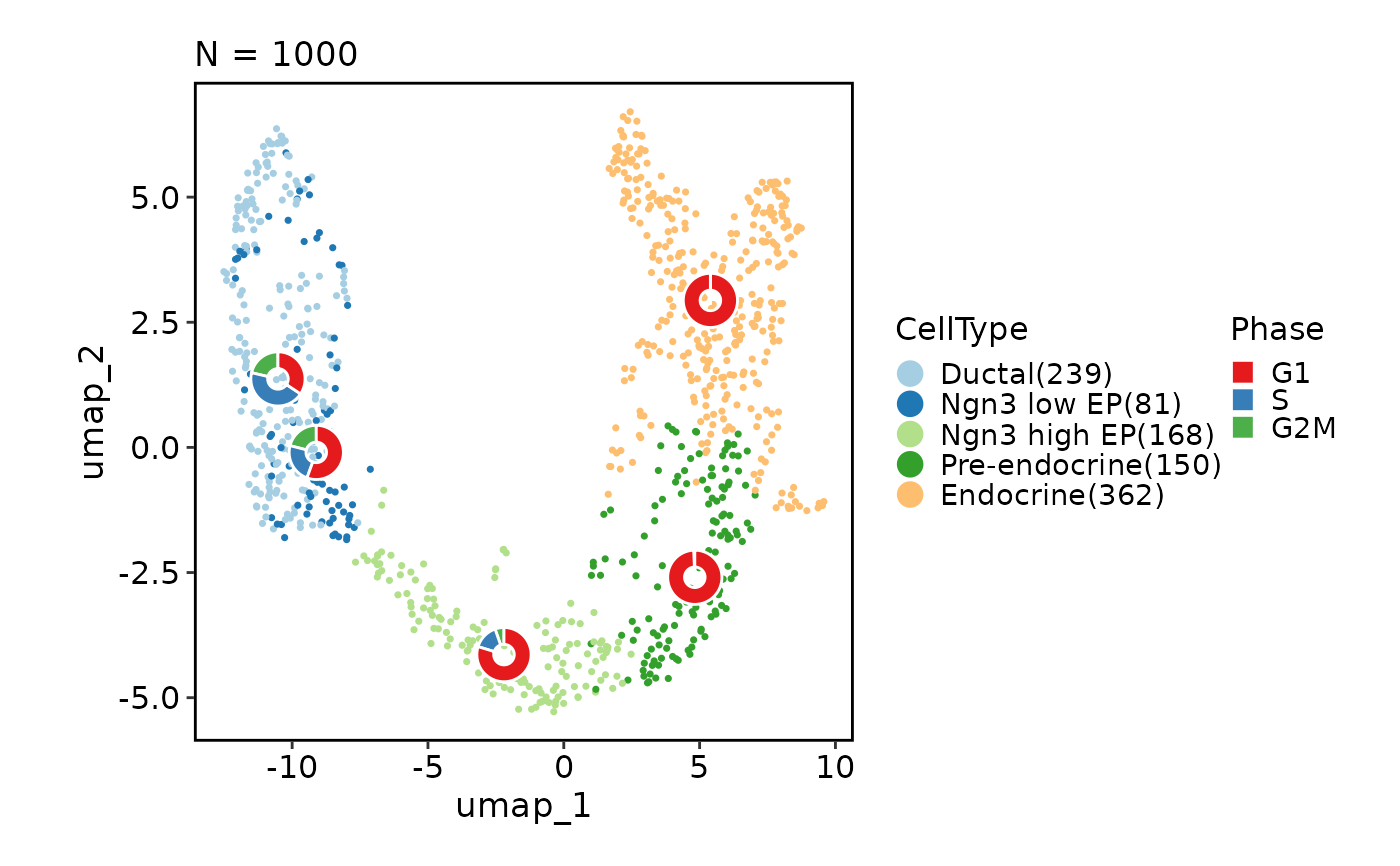
 CellDimPlot(pancreas_sub,
group_by = "CellType", reduction = "UMAP", stat_by = "Phase",
stat_plot_type = "ring", stat_plot_label = TRUE, stat_plot_size = 0.15)
CellDimPlot(pancreas_sub,
group_by = "CellType", reduction = "UMAP", stat_by = "Phase",
stat_plot_type = "ring", stat_plot_label = TRUE, stat_plot_size = 0.15)
 CellDimPlot(pancreas_sub,
group_by = "CellType", reduction = "UMAP", stat_by = "Phase",
stat_plot_type = "bar", stat_type = "count")
CellDimPlot(pancreas_sub,
group_by = "CellType", reduction = "UMAP", stat_by = "Phase",
stat_plot_type = "bar", stat_type = "count")
 CellDimPlot(pancreas_sub,
group_by = "CellType", reduction = "UMAP", stat_by = "Phase",
stat_plot_type = "line", stat_type = "count", stat_args = list(point_size = 1))
#> `geom_line()`: Each group consists of only one observation.
#> ℹ Do you need to adjust the group aesthetic?
#> `geom_line()`: Each group consists of only one observation.
#> ℹ Do you need to adjust the group aesthetic?
CellDimPlot(pancreas_sub,
group_by = "CellType", reduction = "UMAP", stat_by = "Phase",
stat_plot_type = "line", stat_type = "count", stat_args = list(point_size = 1))
#> `geom_line()`: Each group consists of only one observation.
#> ℹ Do you need to adjust the group aesthetic?
#> `geom_line()`: Each group consists of only one observation.
#> ℹ Do you need to adjust the group aesthetic?
 # Chane the plot type from point to the hexagonal bin
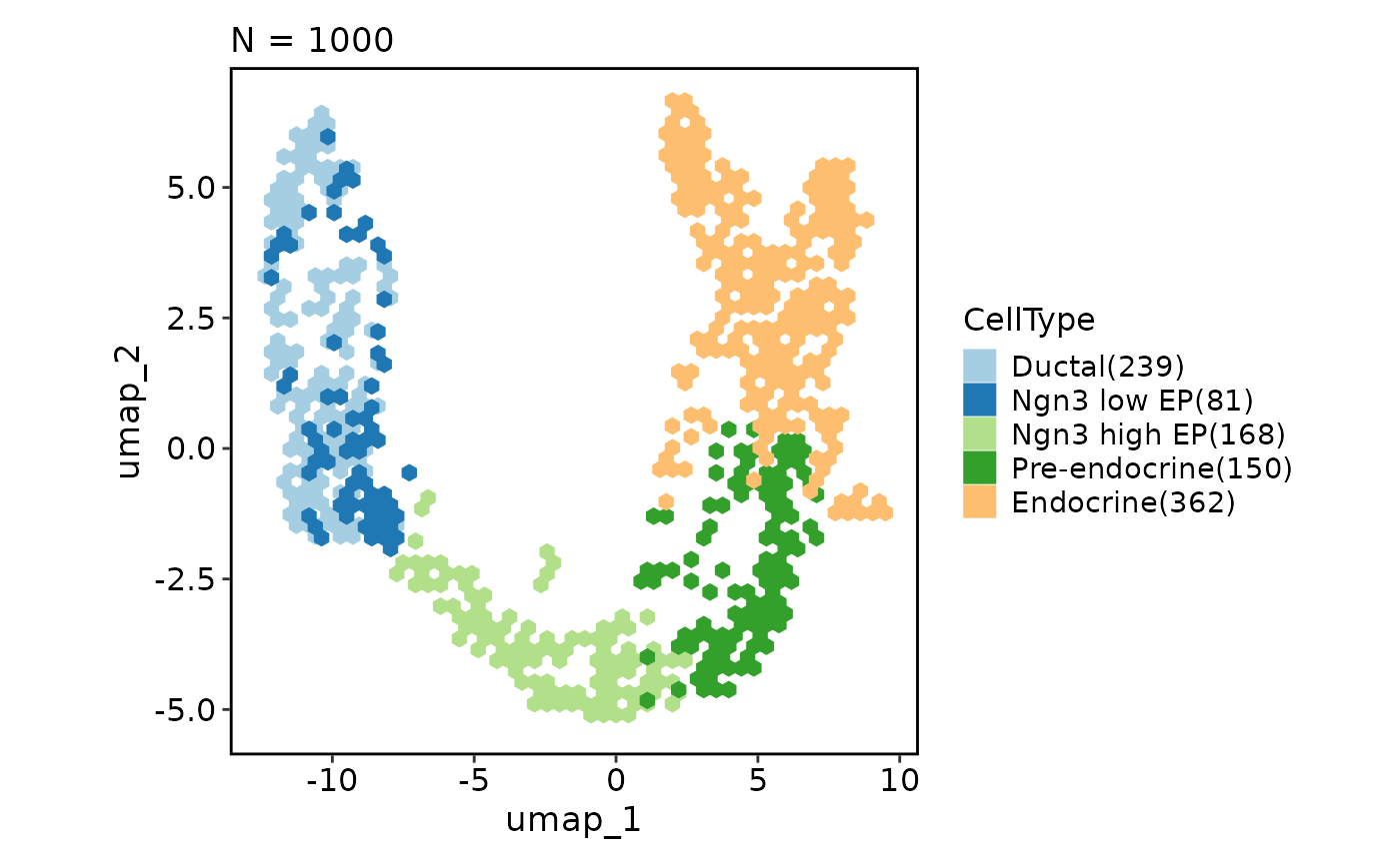
CellDimPlot(pancreas_sub, group_by = "CellType", reduction = "UMAP",
hex = TRUE)
#> Warning: Removed 5 rows containing missing values or values outside the scale range
#> (`geom_hex()`).
# Chane the plot type from point to the hexagonal bin
CellDimPlot(pancreas_sub, group_by = "CellType", reduction = "UMAP",
hex = TRUE)
#> Warning: Removed 5 rows containing missing values or values outside the scale range
#> (`geom_hex()`).
 CellDimPlot(pancreas_sub, group_by = "CellType", reduction = "UMAP",
hex = TRUE, hex_bins = 20)
#> Warning: Removed 4 rows containing missing values or values outside the scale range
#> (`geom_hex()`).
CellDimPlot(pancreas_sub, group_by = "CellType", reduction = "UMAP",
hex = TRUE, hex_bins = 20)
#> Warning: Removed 4 rows containing missing values or values outside the scale range
#> (`geom_hex()`).
 CellDimPlot(pancreas_sub, group_by = "CellType", reduction = "UMAP",
hex = TRUE, hex_count = FALSE)
#> Warning: Removed 5 rows containing missing values or values outside the scale range
#> (`geom_hex()`).
CellDimPlot(pancreas_sub, group_by = "CellType", reduction = "UMAP",
hex = TRUE, hex_count = FALSE)
#> Warning: Removed 5 rows containing missing values or values outside the scale range
#> (`geom_hex()`).
 # Show neighbors graphs on the plot
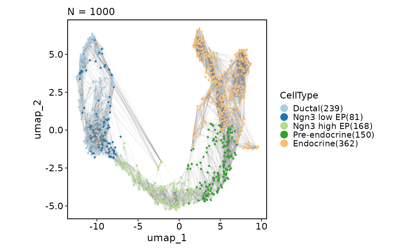
CellDimPlot(pancreas_sub, group_by = "CellType", reduction = "UMAP",
graph = "RNA_nn")
# Show neighbors graphs on the plot
CellDimPlot(pancreas_sub, group_by = "CellType", reduction = "UMAP",
graph = "RNA_nn")
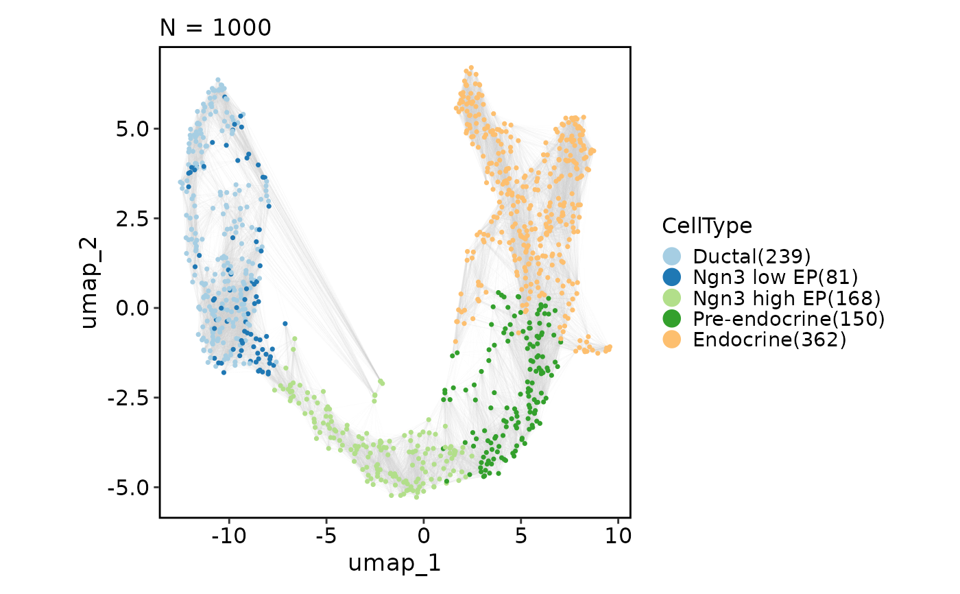
 CellDimPlot(pancreas_sub, group_by = "CellType", reduction = "UMAP",
graph = "RNA_snn", edge_color = "grey80")
CellDimPlot(pancreas_sub, group_by = "CellType", reduction = "UMAP",
graph = "RNA_snn", edge_color = "grey80")
 # Show lineages on the plot based on the pseudotime
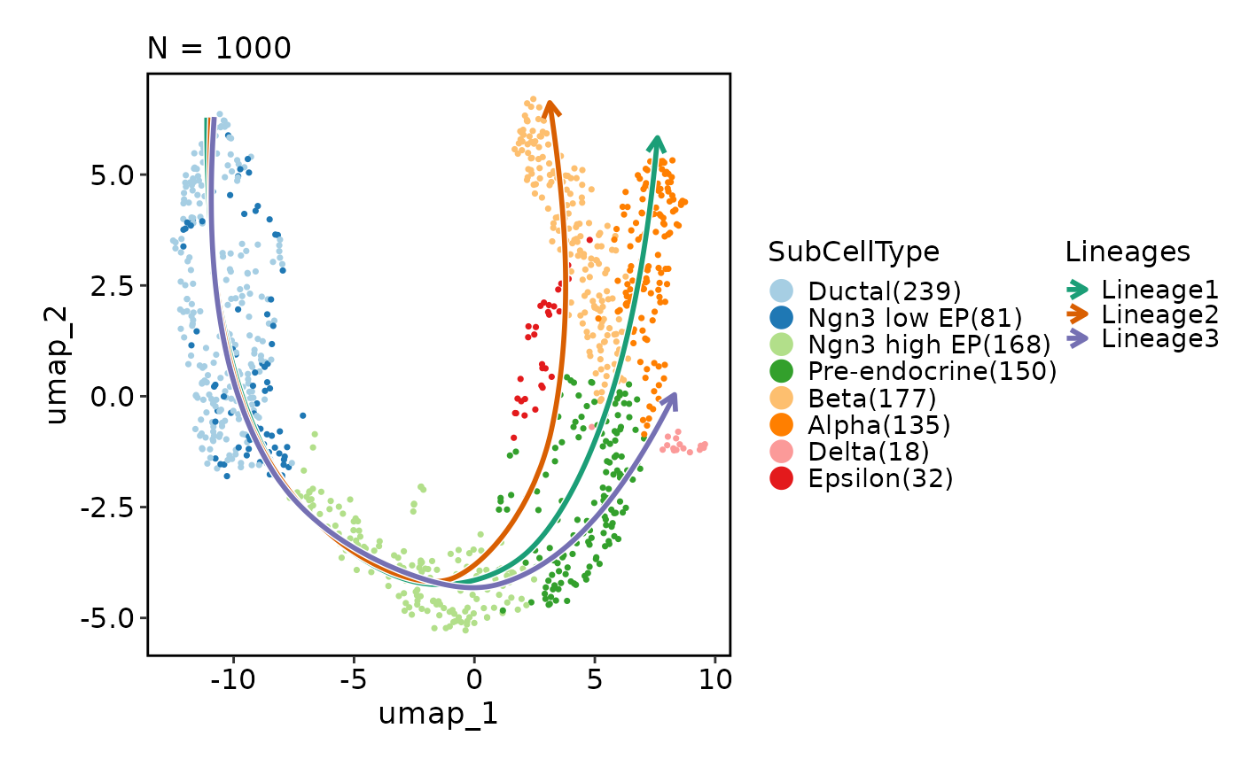
CellDimPlot(pancreas_sub, group_by = "SubCellType", reduction = "UMAP",
lineages = paste0("Lineage", 1:3))
#> Warning: Removed 8 rows containing missing values or values outside the scale range
#> (`geom_path()`).
#> Warning: Removed 8 rows containing missing values or values outside the scale range
#> (`geom_path()`).
# Show lineages on the plot based on the pseudotime
CellDimPlot(pancreas_sub, group_by = "SubCellType", reduction = "UMAP",
lineages = paste0("Lineage", 1:3))
#> Warning: Removed 8 rows containing missing values or values outside the scale range
#> (`geom_path()`).
#> Warning: Removed 8 rows containing missing values or values outside the scale range
#> (`geom_path()`).
 CellDimPlot(pancreas_sub, group_by = "SubCellType", reduction = "UMAP",
lineages = paste0("Lineage", 1:3), lineages_whiskers = TRUE)
#> Warning: Removed 8 rows containing missing values or values outside the scale range
#> (`geom_segment()`).
#> Warning: Removed 8 rows containing missing values or values outside the scale range
#> (`geom_path()`).
#> Warning: Removed 8 rows containing missing values or values outside the scale range
#> (`geom_path()`).
CellDimPlot(pancreas_sub, group_by = "SubCellType", reduction = "UMAP",
lineages = paste0("Lineage", 1:3), lineages_whiskers = TRUE)
#> Warning: Removed 8 rows containing missing values or values outside the scale range
#> (`geom_segment()`).
#> Warning: Removed 8 rows containing missing values or values outside the scale range
#> (`geom_path()`).
#> Warning: Removed 8 rows containing missing values or values outside the scale range
#> (`geom_path()`).
 CellDimPlot(pancreas_sub, group_by = "SubCellType", reduction = "UMAP",
lineages = paste0("Lineage", 1:3), lineages_span = 0.1)
CellDimPlot(pancreas_sub, group_by = "SubCellType", reduction = "UMAP",
lineages = paste0("Lineage", 1:3), lineages_span = 0.1)
 # Velocity
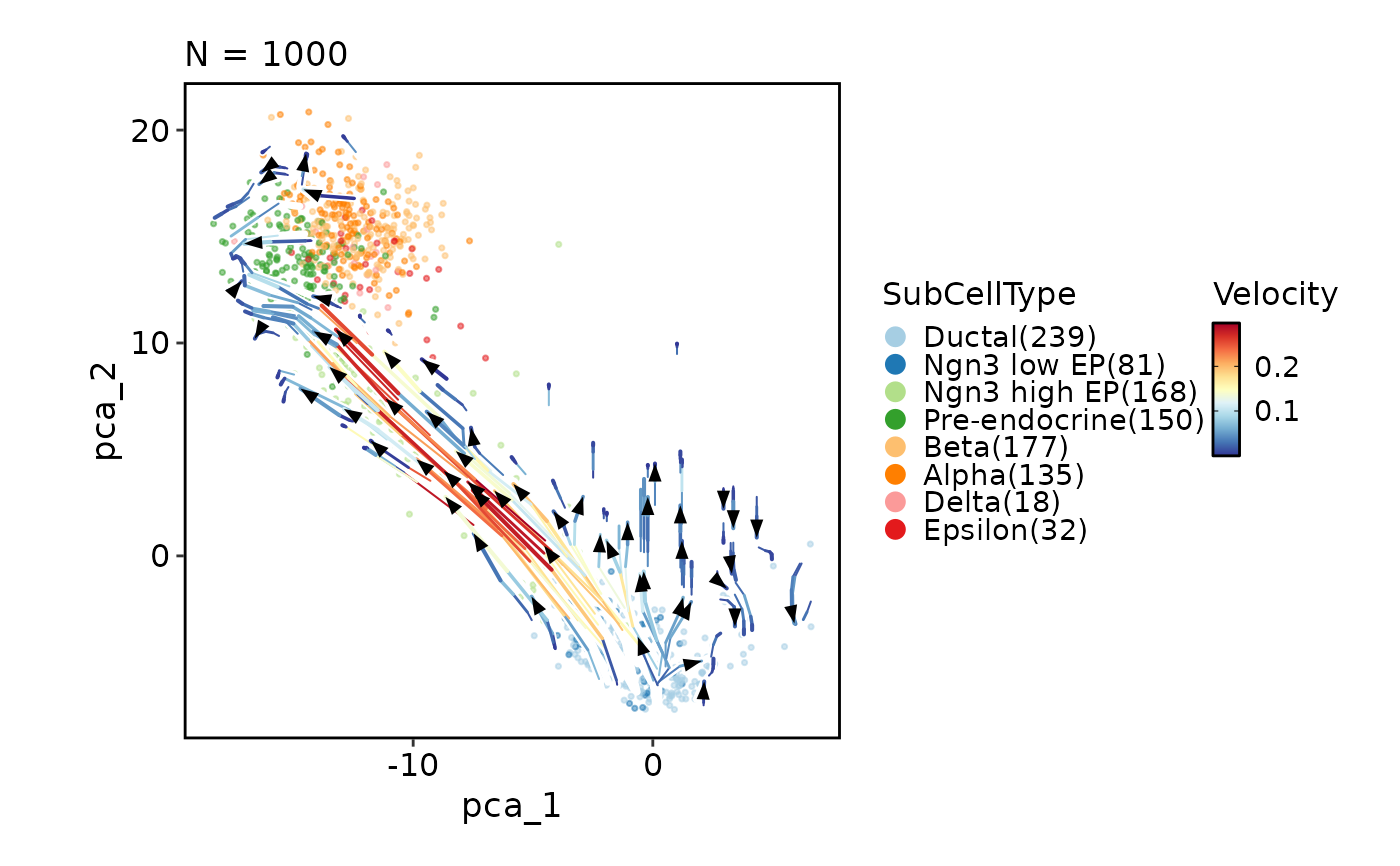
CellDimPlot(pancreas_sub, group_by = "SubCellType", reduction = "PCA",
velocity = "stochastic_PCA")
#> Warning: Removed 2 rows containing missing values or values outside the scale range
#> (`geom_segment()`).
# Velocity
CellDimPlot(pancreas_sub, group_by = "SubCellType", reduction = "PCA",
velocity = "stochastic_PCA")
#> Warning: Removed 2 rows containing missing values or values outside the scale range
#> (`geom_segment()`).
 CellDimPlot(pancreas_sub, group_by = "SubCellType", reduction = "PCA",
velocity = "stochastic_PCA", velocity_plot_type = "grid", pt_alpha = 0.5)
#> Warning: Removed 15 rows containing missing values or values outside the scale range
#> (`geom_segment()`).
CellDimPlot(pancreas_sub, group_by = "SubCellType", reduction = "PCA",
velocity = "stochastic_PCA", velocity_plot_type = "grid", pt_alpha = 0.5)
#> Warning: Removed 15 rows containing missing values or values outside the scale range
#> (`geom_segment()`).
 CellDimPlot(pancreas_sub, group_by = "SubCellType", reduction = "PCA",
velocity = "stochastic_PCA", velocity_plot_type = "stream", pt_alpha = 0.5)
CellDimPlot(pancreas_sub, group_by = "SubCellType", reduction = "PCA",
velocity = "stochastic_PCA", velocity_plot_type = "stream", pt_alpha = 0.5)
 # 3D plot
pancreas_sub@reductions$UMAP@cell.embeddings <- cbind(
pancreas_sub@reductions$UMAP@cell.embeddings,
umap_3 = rnorm(1000) # fake the 3rd dimension
)
CellDimPlot(pancreas_sub, group_by = "SubCellType", reduction = "UMAP",
dims = 1:3, label = TRUE)
# }
# 3D plot
pancreas_sub@reductions$UMAP@cell.embeddings <- cbind(
pancreas_sub@reductions$UMAP@cell.embeddings,
umap_3 = rnorm(1000) # fake the 3rd dimension
)
CellDimPlot(pancreas_sub, group_by = "SubCellType", reduction = "UMAP",
dims = 1:3, label = TRUE)
# }