
DimPlot visualizes dimension reduction data (PCA, t-SNE, UMAP, etc.) as a 2D or 3D
scatter plot. DimPlot() colours points by a discrete grouping variable
(e.g., clusters), while FeatureDimPlot() colours points by a continuous
numeric feature (e.g., gene expression, lineage scores).
Both functions share the same internal engine (DimPlotAtomic) and support
an extensive set of annotation layers: group boundary marks, network/graph
edges, 2D density contours, lineage/trajectory curves, RNA-velocity arrows
(raw, grid, or stream), statistical summary mini-plots at group centroids,
point highlighting, background context points from other facets, and
flexible label positioning.
When dims has 3 elements, both functions automatically return an
interactive plotly 3D scatter plot (via DimPlotAtomic3D). Certain
2D-only features are silently ignored in 3D mode (see @param dims for
the full list).
Rendering scales with dataset size: standard geom_point() for small data,
automatic rasterisation via scattermore::geom_scattermore() when
nrow(data) > 1e5, or hex-bin aggregation (geom_hex() /
stat_summary_hex()).
FeatureDimPlot to visualize feature expression on dimension reduction plots.
Colours points by a
continuous numeric variable (e.g., gene expression, module score, lineage
pseudotime) using a gradient colour scale, with optional quantile trimming
and background cutoff.
When multiple features are provided and facet_by is not set, the data
is automatically pivoted to long format and faceted by feature name.
split_by = TRUE dispatches each feature to a separate plot for
independent layout control. split_by as a column name splits by that
column's levels, producing one plot per level with per-split palette
support.
For detailed split_by workflows, see the main DimPlot / FeatureDimPlot
documentation (@section split_by Workflow (FeatureDimPlot)).
Usage
DimPlot(
  data,
  dims = 1:2,
  group_by,
  group_by_sep = "_",
  split_by = NULL,
  split_by_sep = "_",
  pt_size = NULL,
  pt_alpha = 1,
  bg_color = "grey80",
  label_insitu = FALSE,
  show_stat = !identical(theme, "theme_blank"),
  label = FALSE,
  label_size = 4,
  label_fg = "white",
  label_bg = "black",
  label_bg_r = 0.1,
  label_repel = FALSE,
  label_repulsion = 20,
  label_pt_size = 1,
  label_pt_color = "black",
  label_segment_color = "black",
  order = c("as-is", "reverse", "high-top", "low-top", "random"),
  highlight = NULL,
  highlight_alpha = 1,
  highlight_size = 1,
  highlight_color = "black",
  highlight_stroke = 0.8,
  add_mark = FALSE,
  mark_type = c("hull", "ellipse", "rect", "circle"),
  mark_expand = unit(3, "mm"),
  mark_alpha = 0.1,
  mark_linetype = 1,
  stat_by = NULL,
  stat_plot_type = c("pie", "ring", "bar", "line"),
  stat_plot_size = 0.1,
  stat_args = list(palette = "Set1"),
  graph = NULL,
  edge_size = c(0.05, 0.5),
  edge_alpha = 0.1,
  edge_color = "grey40",
  add_density = FALSE,
  density_color = "grey80",
  density_filled = FALSE,
  density_filled_palette = "Greys",
  density_filled_palcolor = NULL,
  lineages = NULL,
  lineages_trim = c(0.01, 0.99),
  lineages_span = 0.75,
  lineages_palette = "Dark2",
  lineages_palcolor = NULL,
  lineages_arrow = arrow(length = unit(0.1, "inches")),
  lineages_linewidth = 1,
  lineages_line_bg = "white",
  lineages_line_bg_stroke = 0.5,
  lineages_whiskers = FALSE,
  lineages_whiskers_linewidth = 0.5,
  lineages_whiskers_alpha = 0.5,
  velocity = NULL,
  velocity_plot_type = c("raw", "grid", "stream"),
  velocity_n_neighbors = NULL,
  velocity_density = 1,
  velocity_smooth = 0.5,
  velocity_scale = 1,
  velocity_min_mass = 1,
  velocity_cutoff_perc = 5,
  velocity_group_palette = "Set2",
  velocity_group_palcolor = NULL,
  arrow_angle = 20,
  arrow_color = "black",
  arrow_alpha = 1,
  streamline_l = 5,
  streamline_minl = 1,
  streamline_res = 1,
  streamline_n = 15,
  streamline_width = c(0, 0.8),
  streamline_alpha = 1,
  streamline_color = NULL,
  streamline_palette = "RdYlBu",
  streamline_palcolor = NULL,
  streamline_bg_color = "white",
  streamline_bg_stroke = 0.5,
  keep_na = FALSE,
  keep_empty = FALSE,
  facet_by = NULL,
  facet_scales = "fixed",
  facet_nrow = NULL,
  facet_ncol = NULL,
  facet_byrow = TRUE,
  title = NULL,
  subtitle = NULL,
  xlab = NULL,
  ylab = NULL,
  theme = "theme_this",
  theme_args = list(),
  aspect.ratio = 1,
  legend.position = "right",
  legend.direction = "vertical",
  raster = NULL,
  raster_dpi = c(512, 512),
  hex = FALSE,
  hex_linewidth = 0.5,
  hex_count = TRUE,
  hex_bins = 50,
  hex_binwidth = NULL,
  palette = "Paired",
  palcolor = NULL,
  palreverse = FALSE,
  seed = 8525,
  combine = TRUE,
  nrow = NULL,
  ncol = NULL,
  byrow = TRUE,
  axes = NULL,
  axis_titles = axes,
  guides = NULL,
  design = NULL,
  ...
)

FeatureDimPlot(
  data,
  dims = 1:2,
  features,
  split_by = NULL,
  split_by_sep = "_",
  lower_quantile = 0,
  upper_quantile = 0.99,
  lower_cutoff = NULL,
  upper_cutoff = NULL,
  pt_size = NULL,
  pt_alpha = 1,
  bg_color = "grey80",
  bg_cutoff = NULL,
  label_insitu = FALSE,
  show_stat = !identical(theme, "theme_blank"),
  color_name = "",
  label = FALSE,
  label_size = 4,
  label_fg = "white",
  label_bg = "black",
  label_bg_r = 0.1,
  label_repel = FALSE,
  label_repulsion = 20,
  label_pt_size = 1,
  label_pt_color = "black",
  label_segment_color = "black",
  order = c("as-is", "reverse", "high-top", "low-top", "random"),
  highlight = NULL,
  highlight_alpha = 1,
  highlight_size = 1,
  highlight_color = "black",
  highlight_stroke = 0.8,
  add_mark = FALSE,
  mark_type = c("hull", "ellipse", "rect", "circle"),
  mark_expand = unit(3, "mm"),
  mark_alpha = 0.1,
  mark_linetype = 1,
  keep_na = FALSE,
  keep_empty = FALSE,
  stat_by = NULL,
  stat_plot_type = c("pie", "ring", "bar", "line"),
  stat_plot_size = 0.1,
  stat_args = list(palette = "Set1"),
  graph = NULL,
  edge_size = c(0.05, 0.5),
  edge_alpha = 0.1,
  edge_color = "grey40",
  add_density = FALSE,
  density_color = "grey80",
  density_filled = FALSE,
  density_filled_palette = "Greys",
  density_filled_palcolor = NULL,
  lineages = NULL,
  lineages_trim = c(0.01, 0.99),
  lineages_span = 0.75,
  lineages_palette = "Dark2",
  lineages_palcolor = NULL,
  lineages_arrow = arrow(length = unit(0.1, "inches")),
  lineages_linewidth = 1,
  lineages_line_bg = "white",
  lineages_line_bg_stroke = 0.5,
  lineages_whiskers = FALSE,
  lineages_whiskers_linewidth = 0.5,
  lineages_whiskers_alpha = 0.5,
  velocity = NULL,
  velocity_plot_type = c("raw", "grid", "stream"),
  velocity_n_neighbors = NULL,
  velocity_density = 1,
  velocity_smooth = 0.5,
  velocity_scale = 1,
  velocity_min_mass = 1,
  velocity_cutoff_perc = 5,
  velocity_group_palette = "Set2",
  velocity_group_palcolor = NULL,
  arrow_angle = 20,
  arrow_color = "black",
  arrow_alpha = 1,
  streamline_l = 5,
  streamline_minl = 1,
  streamline_res = 1,
  streamline_n = 15,
  streamline_width = c(0, 0.8),
  streamline_alpha = 1,
  streamline_color = NULL,
  streamline_palette = "RdYlBu",
  streamline_palcolor = NULL,
  streamline_bg_color = "white",
  streamline_bg_stroke = 0.5,
  facet_by = NULL,
  facet_scales = "fixed",
  facet_nrow = NULL,
  facet_ncol = NULL,
  facet_byrow = TRUE,
  title = NULL,
  subtitle = NULL,
  xlab = NULL,
  ylab = NULL,
  theme = "theme_this",
  theme_args = list(),
  aspect.ratio = 1,
  legend.position = "right",
  legend.direction = "vertical",
  raster = NULL,
  raster_dpi = c(512, 512),
  hex = FALSE,
  hex_linewidth = 0.5,
  hex_count = FALSE,
  hex_bins = 50,
  hex_binwidth = NULL,
  palette = "Spectral",
  palcolor = NULL,
  palreverse = FALSE,
  seed = 8525,
  combine = TRUE,
  nrow = NULL,
  ncol = NULL,
  byrow = TRUE,
  axes = NULL,
  axis_titles = axes,
  guides = NULL,
  design = NULL,
  ...
)
Arguments
- data
A data frame.
- dims
A character vector of the column names to plot on the x, y (and optionally z) axes or a numeric vector of the column indices. When 3 dimensions are provided, a 3D interactive plot is created using plotly. Supported in 3D: group_by, features, labels, highlight, lineages, graph/network, show_stat, order. Not supported in 3D: add_mark, stat_by, add_density, velocity, hex, facet_by, raster.
- group_by
Columns to group the data for plotting For those plotting functions that do not support multiple groups, They will be concatenated into one column, using
group_by_sepas the separator- group_by_sep
The separator for multiple group_by columns. See
group_by- split_by
A character vector of column names to split the data by and plot separately. If
TRUE, the data is split byfeatures— each feature is plotted in its own panel. Use this instead offacet_bywhen you need independent layout control (nrow,ncol) or per-feature palettes viasplit_by = TRUEcombined withpalette/palcolor.- split_by_sep
The separator for multiple split_by columns. See
split_by- pt_size
A numeric value for point size, or a character string naming a numeric column in
datato map point sizes to. IfNULL(default), auto-calculated asmin(3000 / nrow(data), 0.6). Column-name mapping only applies to 2D plots and is ignored with a message whenraster = TRUE.- pt_alpha
A numeric value in
[0, 1]for the point transparency. Default is1.- bg_color
A character string specifying the colour used for NA-valued points and background context points drawn from other facets. Default is
"grey80".- label_insitu
A logical value. If
TRUE, the raw group names are placed at the group median coordinates instead of numeric indices. Forceslabel = TRUE. Default isFALSE.- show_stat
A logical value. If
TRUE(default), the number of points per group is shown in the legend labels and subtitle. Ignored whentheme = "theme_blank".- label
A logical value. If
TRUE, group labels (numeric indices by default, or group names whenlabel_insitu = TRUE) are placed at the median coordinates of each group. Forced toTRUEwhenlabel_repelorlabel_insituis set.- label_size
A numeric value for the label text size. Passed to
ggrepel::geom_text_repel(). Default is4.- label_fg
A character string for the label text (foreground) colour. Default is
"white".- label_bg
A character string for the label background / outline colour. Default is
"black".- label_bg_r
A numeric value for the background fill ratio of the label bounding box. Passed to
ggrepel::geom_text_repel(bg.r = ...). Default is0.1.- label_repel
A logical value. If
TRUE, labels are repelled from each other with forcelabel_repulsion. A visible point anchor is drawn. Forceslabel = TRUE.- label_repulsion
A numeric value for the repulsion force when
label_repel = TRUE. Passed toggrepel::geom_text_repel(force = ...). Default is20.- label_pt_size
A numeric value for the size of the anchor point drawn when
label_repel = TRUE. Default is1.- label_pt_color
A character string for the colour of the label anchor point. Default is
"black".- label_segment_color
A character string for the colour of the line segment connecting the label to the anchor. Used in non-repel mode (
label_repel = FALSE) wheremin.segment.length = 0. Default is"black".- order
A character string controlling the draw order of points:
"as-is"(default) — the row order in the data is preserved."reverse"— rows are reversed."high-top"— points with high values (last factor levels for group_by) are drawn last (on top)."low-top"— points with low values (first factor levels) are drawn last."random"— rows are randomly shuffled.
For
high-topandlow-top, NA values are always plotted at the bottom. When applied togroup_by, only the draw order changes — legend colours and order are unaffected. Within the same level, point order is preserved. For precise control, set factor levels before plotting. See https://github.com/pwwang/scplotter/issues/29#issuecomment-3009694130 for examples.- highlight
A specification for highlighted points:
NULL(default): no highlighting.TRUE: highlight all points (adds a dark outline around every point).A character string: a dplyr filter expression (e.g.,
"clusters == 'Ductal'").A character vector: row names to highlight.
A numeric vector: row indices to highlight.
- highlight_alpha
A numeric value in
[0, 1]for the transparency of highlighted points. Default is1.- highlight_size
A numeric value for the size of the inner (coloured) highlight point. Default is
1.- highlight_color
A character string for the colour of the outer highlight ring. Default is
"black".- highlight_stroke
A numeric value for the thickness of the outer highlight ring (the difference between the outer ring size and
highlight_size). Default is0.8.- add_mark
A logical value. If
TRUE, group boundaries are drawn around points usingggforcemarks. Requiresgroup_by. Only supported in 2D.- mark_type
A character string specifying the mark shape. Options:
"hull"(convex hull, default),"ellipse","rect", or"circle".- mark_expand
A unit value for the outward expansion of the mark boundary. Passed to
ggforce::geom_mark_*(expand = ...). Default isunit(3, "mm").- mark_alpha
A numeric value in
[0, 1]for the transparency of the mark fill. Default is0.1.- mark_linetype
A numeric value for the line type of the mark boundary. Default is
1(solid).- stat_by
A character string naming a column used to compute per-group statistical summary mini-plots embedded at group centroid positions. Only supported with
group_by(notfeatures). Only supported in 2D withoutfacet_by.- stat_plot_type
A character string specifying the mini-plot type. Options:
"pie"(default),"ring","bar", or"line".- stat_plot_size
A numeric value for the size of the stat mini-plot, expressed as a fraction of the axis range. Default is
0.1.- stat_args
A list of additional arguments passed to the stat plot function (e.g.,
list(palette = "Set1")). Default islist(palette = "Set1").- graph
A specification for network / graph edges to overlay. Sources:
A character string starting with
"@"(e.g.,"@graph"): extracts the attribute named"graph"fromattributes(data).A
Graphobject (e.g., Seurat): coerced to dense matrix viaas.matrix().A
matrix,data.frame, ordgCMatrix: used directly as the adjacency matrix.Numeric indices or character column names: extracts columns from
data. Edges are drawn for non-zero, lower-triangle entries. Requiresdatato have row names matching the matrix dimnames.
- edge_size
A numeric vector of length 2 specifying the range
[min, max]forscale_linewidth_continuous(range = ...)applied to edge widths. Default isc(0.05, 0.5).- edge_alpha
A numeric value in
[0, 1]for the transparency of graph edges. Default is0.1.- edge_color
A character string for the colour of graph edges. Default is
"grey40".- add_density
A logical value. If
TRUE, a 2D density layer is overlaid. Only supported in 2D.- density_color
A character string for the colour of the density contour lines. Used when
density_filled = FALSE. Default is"grey80".- density_filled
A logical value. If
TRUE, the density is rendered as a filled raster (stat_density_2d(geom = "raster")) instead of contour lines. A separate fill scale is used.- density_filled_palette
A character string naming the palette for the filled density layer. Default is
"Greys".- density_filled_palcolor
A character vector of specific colours for the filled density palette. Default is
NULL(auto-resolved fromdensity_filled_palette).- lineages
A character vector of column names representing pseudotime / trajectory lineages. Each column is fitted with a LOESS smooth (
span = lineages_span, degree = 2) across the 2D embedding, after trimming the top and bottomlineages_trimquantiles. Only supported in 2D withoutfacet_by.- lineages_trim
A numeric vector of length 2 specifying the lower and upper quantile thresholds
[0, 1]for trimming lineage values before LOESS fitting. Default isc(0.01, 0.99).- lineages_span
A numeric value passed as
spantostats::loess()controlling the smoothness of the lineage curve. Smaller values follow the data more closely. Default is0.75.- lineages_palette
A character string naming the palette for lineage colours. Default is
"Dark2".- lineages_palcolor
A character vector of specific colours for lineage curves. Default is
NULL(auto-resolved fromlineages_palette).- lineages_arrow
A ggplot2
arrowspecification applied to the end of lineage paths. Default isarrow(length = unit(0.1, "inches")).- lineages_linewidth
A numeric value for the width of the lineage curve lines. Default is
1.- lineages_line_bg
A character string for the colour of the background (wider) stroke drawn behind each lineage curve for improved visibility. Default is
"white".- lineages_line_bg_stroke
A numeric value for the additional width of the background stroke relative to
lineages_linewidth. The background line has total widthlineages_linewidth + lineages_line_bg_stroke. Default is0.5.- lineages_whiskers
A logical value. If
TRUE, short line segments connect the smoothed lineage curve to the original data coordinates of the fitted points. Default isFALSE.- lineages_whiskers_linewidth
A numeric value for the width of the whisker lines. Default is
0.5.- lineages_whiskers_alpha
A numeric value in
[0, 1]for the transparency of the whisker lines. Default is0.5.- velocity
A specification for RNA-velocity arrows. Can be:
NULL(default): no velocity overlay.A character / integer vector: column names or indices in
datafor the velocity embedding.A data frame or matrix: the velocity embedding itself (must align with
datarows). Only supported in 2D withoutfacet_by.
- velocity_plot_type
A character string specifying the velocity rendering style. Options:
"raw"(arrows from embedding),"grid"(grid-based arrows), or"stream"(streamlines). Default is"raw".- velocity_n_neighbors
A numeric value for the number of neighbours used in the velocity grid computation. Default is
NULL(auto).- velocity_density
A numeric value for the velocity kernel density bandwidth. Default is
1.- velocity_smooth
A numeric value for the velocity smoothing parameter. Default is
0.5.- velocity_scale
A numeric value for scaling the velocity arrows. Default is
1.- velocity_min_mass
A numeric value for the minimum cell mass threshold in velocity grid computation. Default is
1.- velocity_cutoff_perc
A numeric value for the velocity cutoff percentage. Default is
5.- velocity_group_palette
A character string naming the palette for velocity group colours (used in
"raw"plot type). Default is"Set2".- velocity_group_palcolor
A character vector of specific colours for velocity groups. Default is
NULL(auto-resolved fromvelocity_group_palette).- arrow_angle
A numeric value specifying the angle of the arrowheads in degrees. Applied to
arrowwhenplot_typeis"raw"or"grid". Default is 20.- arrow_color
A character string specifying the color of the velocity arrows. For
plot_type = "stream", this sets only the arrowhead color. Default is"black".- arrow_alpha
A numeric value between 0 and 1 specifying the transparency of the velocity arrows. Only used when
plot_type = "raw"or"grid"; forplot_type = "stream", usestreamline_alphainstead. Default is 1.- streamline_l
A numeric value specifying the integration length of the streamlines. Passed to
geom_streamlineas theLparameter. Default is 5.- streamline_minl
A numeric value specifying the minimum streamline length. Shorter streamlines are not drawn. Passed to
geom_streamlineas themin.Lparameter. Default is 1.- streamline_res
A numeric value specifying the resolution of the streamline integration. Passed to
geom_streamlineas theresparameter. Default is 1.- streamline_n
A numeric value specifying the number of streamlines to draw. Passed to
geom_streamlineas thenparameter. Default is 15.- streamline_width
A numeric vector of length 2 specifying the range of line widths for streamlines. Passed to
scale_size(range = ...). Only used whenstreamline_colorisNULL. Default isc(0, 0.8).- streamline_alpha
A numeric value between 0 and 1 specifying the transparency of the velocity streamlines. Default is 1.
- streamline_color
An optional character string specifying a fixed color for streamlines. When
NULL(the default), streamlines are colored by velocity magnitude usingstreamline_palette.- streamline_palette
A character string specifying the color palette for streamline velocity magnitude. Passed to
palette_this. Only used whenstreamline_colorisNULL. Default is"RdYlBu".- streamline_palcolor
An optional character vector of specific colors for the streamline velocity gradient. If
NULL, colors are generated fromstreamline_palette. Default isNULL.- streamline_bg_color
A character string specifying the background (outline) color applied to streamlines to create a stroke effect. Default is
"white".- streamline_bg_stroke
A numeric value specifying the additional line width of the background stroke relative to the foreground streamline. Default is 0.5.
- keep_na
A logical value or a character to replace the NA values in the data. It can also take a named list to specify different behavior for different columns. If TRUE or NA, NA values will be replaced with NA. If FALSE, NA values will be removed from the data before plotting. If a character string is provided, NA values will be replaced with the provided string. If a named vector/list is provided, the names should be the column names to apply the behavior to, and the values should be one of TRUE, FALSE, or a character string. Without a named vector/list, the behavior applies to categorical/character columns used on the plot, for example, the
x,group_by,fill_by, etc.- keep_empty
One of FALSE, TRUE and "level". It can also take a named list to specify different behavior for different columns. Without a named list, the behavior applies to the categorical/character columns used on the plot, for example, the
x,group_by,fill_by, etc.FALSE(default): Drop empty factor levels from the data before plotting.TRUE: Keep empty factor levels and show them as a separate category in the plot."level": Keep empty factor levels, but do not show them in the plot. But they will be assigned colors from the palette to maintain consistency across multiple plots. Alias:levels
- facet_by
A character string specifying the column name of the data frame to facet the plot. Otherwise, the data will be split by
split_byand generate multiple plots and combine them into one usingpatchwork::wrap_plots- facet_scales
Whether to scale the axes of facets. Default is "fixed" Other options are "free", "free_x", "free_y". See
ggplot2::facet_wrap- facet_nrow
A numeric value specifying the number of rows in the facet. When facet_by is a single column and facet_wrap is used.
- facet_ncol
A numeric value specifying the number of columns in the facet. When facet_by is a single column and facet_wrap is used.
- facet_byrow
A logical value indicating whether to fill the plots by row. Default is TRUE.
- title
A character string specifying the title of the plot. A function can be used to generate the title based on the default title. This is useful when split_by is used and the title needs to be dynamic.
- subtitle
A character string specifying the subtitle of the plot.
- xlab
A character string specifying the x-axis label.
- ylab
A character string specifying the y-axis label.
- theme
A character string or a theme class (i.e. ggplot2::theme_classic) specifying the theme to use. Default is "theme_this".
- theme_args
A list of arguments to pass to the theme function.
- aspect.ratio
A numeric value specifying the aspect ratio of the plot.
- legend.position
A character string specifying the position of the legend. if
waiver(), for single groups, the legend will be "none", otherwise "right".- legend.direction
A character string specifying the direction of the legend.
- raster
A logical value. If
TRUE, points are rendered viascattermore::geom_scattermore()for efficient rasterised plotting. Default isNULL, which auto-enables whennrow(data) > 1e5.- raster_dpi
A numeric vector of length 2
[x_dpi, y_dpi]specifying the raster resolution in pixels. Passed toscattermore::geom_scattermore(pixels = ...). Default isc(512, 512). If a single value is provided it is recycled to both dimensions.- hex
A logical value. If
TRUE, points are rendered as hexagonal bins viageom_hex()/stat_summary_hex(). Not supported with highlight. Default isFALSE. Only supported in 2D.- hex_linewidth
A numeric value for the width of the hexagon boundary lines. Default is
0.5.- hex_count
A logical value. If
TRUEandgroup_byis set, hex fill alpha is mapped toafter_stat(count)so denser bins are more opaque. Forfeaturesmode hex_count is ignored. Default is!is.null(group_by).- hex_bins
A numeric value for the number of hex bins along each axis. Passed to
geom_hex(bins = ...). Default is50.- hex_binwidth
A numeric value for the width of individual hex bins. Passed to
geom_hex(binwidth = ...). Takes precedence overhex_binswhen set.- palette
A character string specifying the palette to use. A named list or vector can be used to specify the palettes for different
split_byvalues.- palcolor
A character string specifying the color to use in the palette. A named list can be used to specify the colors for different
split_byvalues. If some values are missing, the values from the palette will be used (palcolor will be NULL for those values).- palreverse
A logical value indicating whether to reverse the palette. Default is FALSE.
- seed
The random seed to use. Default is 8525.
- combine
Whether to combine the plots into one when facet is FALSE. Default is TRUE.
- nrow
A numeric value specifying the number of rows in the facet.
- ncol
A numeric value specifying the number of columns in the facet.
- byrow
A logical value indicating whether to fill the plots by row.
- axes
A string specifying how axes should be treated. Passed to
patchwork::wrap_plots(). Only relevant whensplit_byis used andcombineis TRUE. Options are:'keep' will retain all axes in individual plots.
'collect' will remove duplicated axes when placed in the same run of rows or columns of the layout.
'collect_x' and 'collect_y' will remove duplicated x-axes in the columns or duplicated y-axes in the rows respectively.
- axis_titles
A string specifying how axis titltes should be treated. Passed to
patchwork::wrap_plots(). Only relevant whensplit_byis used andcombineis TRUE. Options are:'keep' will retain all axis titles in individual plots.
'collect' will remove duplicated titles in one direction and merge titles in the opposite direction.
'collect_x' and 'collect_y' control this for x-axis titles and y-axis titles respectively.
- guides
A string specifying how guides should be treated in the layout. Passed to
patchwork::wrap_plots(). Only relevant whensplit_byis used andcombineis TRUE. Options are:'collect' will collect guides below to the given nesting level, removing duplicates.
'keep' will stop collection at this level and let guides be placed alongside their plot.
'auto' will allow guides to be collected if a upper level tries, but place them alongside the plot if not.
- design
Specification of the location of areas in the layout, passed to
patchwork::wrap_plots(). Only relevant whensplit_byis used andcombineis TRUE. When specified,nrow,ncol, andbyroware ignored. Seepatchwork::wrap_plots()for more details.- ...
Additional arguments.
- features
A character vector of the column names to plot as features (continuous colouring). When multiple features are provided and
facet_byis not set, the data is pivoted to long format and faceted by feature name.- lower_quantile, upper_quantile
Lower and upper quantiles for the continuous color/fill scale. The actual cutoffs are determined by these quantiles when
lower_cutoffandupper_cutoffareNULL. Defaults:lower_quantile = 0,upper_quantile = 0.99.- lower_cutoff, upper_cutoff
Explicit lower and upper cutoffs for the continuous color/fill scale. When
NULL(the default), the cutoffs are determined bylower_quantileandupper_quantileviaquantile. Values outside the[lower_cutoff, upper_cutoff]range are clamped (winsorized) to the nearest cutoff value.- bg_cutoff
A numeric threshold. Feature values with absolute value below this cutoff are set to
NA(and therefore rendered inbg_color). Default isNULL.- color_name
A character string used as the title for the continuous colour bar in feature mode. Default is
"".
Value
A ggplot object (single plot), a patchwork / wrap_plots object
(when split_by is provided and combine = TRUE), or a list of ggplot
objects (when split_by is provided and combine = FALSE).
When dims has 3 elements, a plotly object is returned instead.
A ggplot object (single plot), a patchwork / wrap_plots object
(when split_by is provided and combine = TRUE), or a list of ggplot
objects (when split_by is provided and combine = FALSE).
When dims has 3 elements, a plotly object is returned instead.
split_by Workflow (DimPlot)
When split_by is specified, DimPlot() executes the following pipeline:
Argument validation —
validate_common_args()checks the seed and blockssplit_by+velocitycombinations.NA / empty normalisation —
check_keep_na()/check_keep_empty()convertkeep_na/keep_emptyto per-column lists.Theme resolution —
process_theme()resolves the theme string to a theme function.Split column resolution —
check_columns()validatessplit_by(force_factor, concat_multi).Pre-filtering —
process_keep_na_empty()removes NA / empty levels from the split column, thendatais split bysplit_bylevels (order preserved). Whengraphreferences an attribute (@graph), the graph matrix is also subset per split.Per-split parameter resolution —
check_palette(),check_palcolor(),check_legend()resolve palette, palcolor, legend.position, and legend.direction for each split.Per-split dispatch — each split is passed to
DimPlotAtomic()with its resolved parameters. Title defaults to the split level name unlesstitleis a function.Combination —
combine_plots()assembles the list of plots viapatchwork::wrap_plots(), applyingnrow,ncol,byrow,axes,axis_titles,guides, anddesign.
split_by Workflow (FeatureDimPlot)
FeatureDimPlot() supports two forms of splitting:
A. split_by = TRUE (split by features)
Each feature in
featuresis dispatched individually toDimPlotAtomic(), producing one plot per feature. The plot title defaults to the feature name.Plots are combined via
combine_plots()withsplit_by = ".features".
B. split_by as a column name (split by data column)
Data is split by the named column's levels (same pipeline as DimPlot steps 1–8 above). Graph attribute splitting is supported.
Examples
# \donttest{
data(dim_example)
# basic dim plot
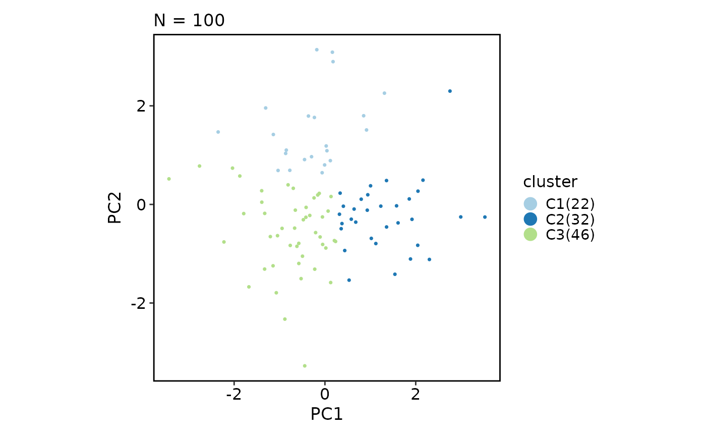
DimPlot(dim_example, group_by = "clusters")
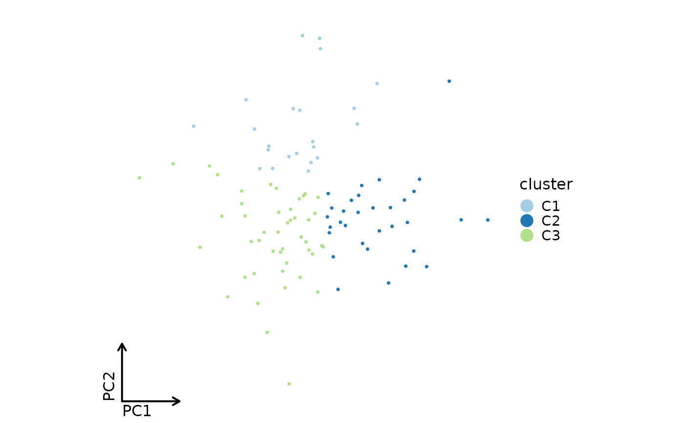
 DimPlot(dim_example, group_by = "clusters", theme = "theme_blank")
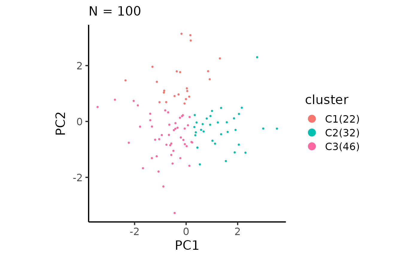
 DimPlot(dim_example, group_by = "clusters", theme = ggplot2::theme_classic,
theme_args = list(base_size = 16), palette = "seurat")
DimPlot(dim_example, group_by = "clusters", theme = ggplot2::theme_classic,
theme_args = list(base_size = 16), palette = "seurat")
 # raster and highlighting
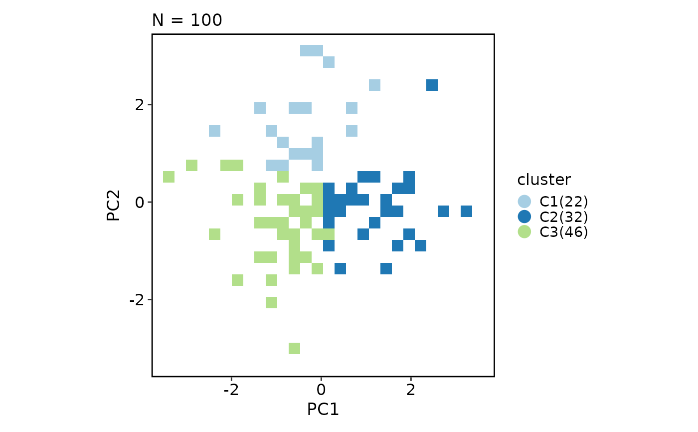
DimPlot(dim_example, group_by = "clusters", raster = TRUE, raster_dpi = 50)
# raster and highlighting
DimPlot(dim_example, group_by = "clusters", raster = TRUE, raster_dpi = 50)
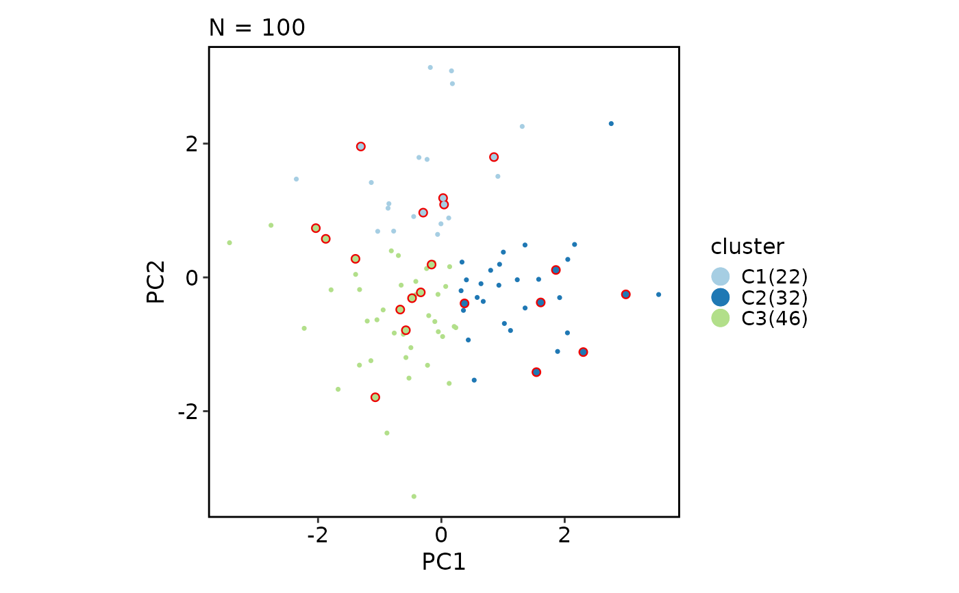
 DimPlot(dim_example, group_by = "clusters", highlight = 1:20,
highlight_color = "black", highlight_stroke = 2)
DimPlot(dim_example, group_by = "clusters", highlight = 1:20,
highlight_color = "black", highlight_stroke = 2)
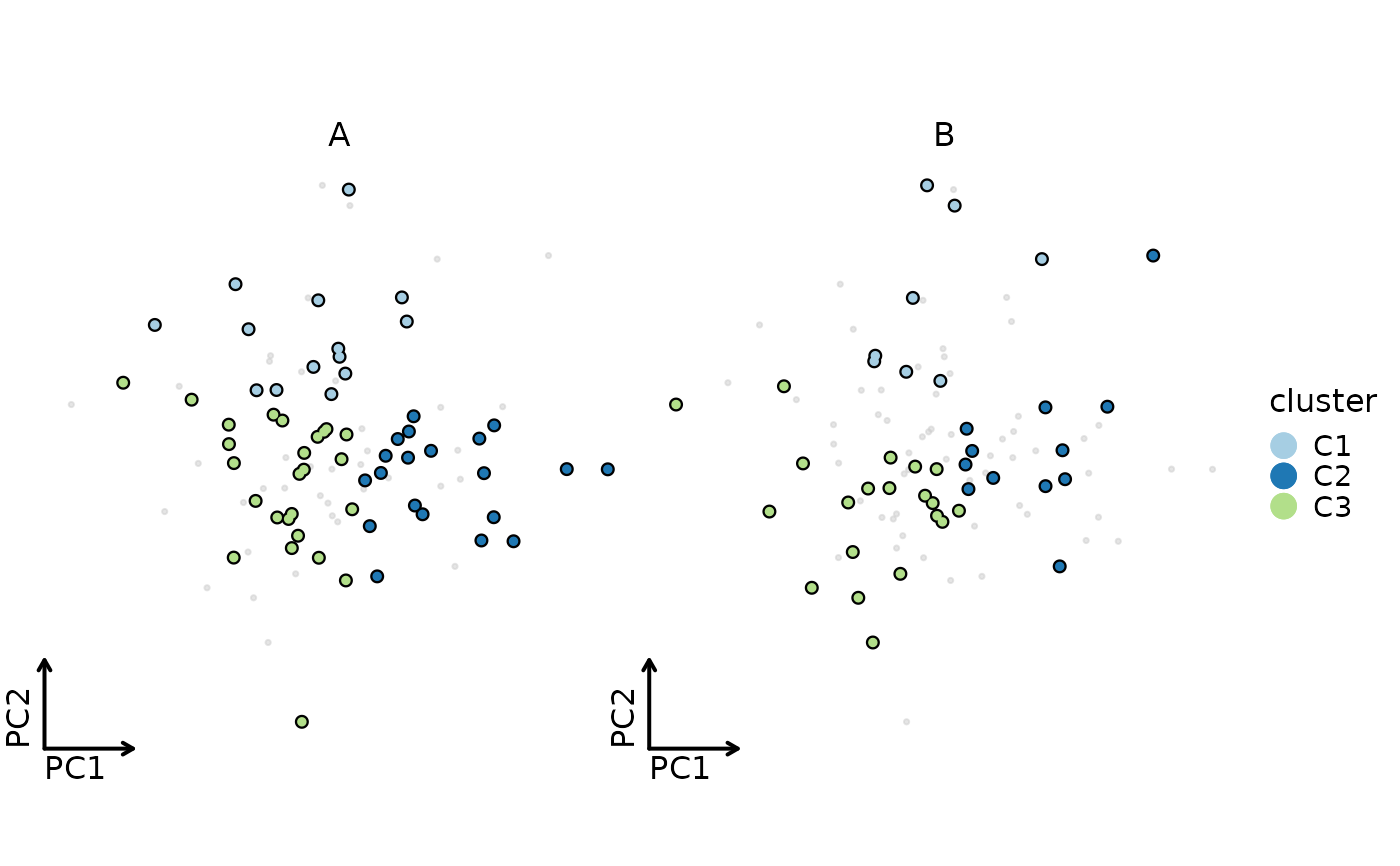
 DimPlot(dim_example, group_by = "clusters", highlight = TRUE, facet_by = "group",
theme = "theme_blank")
DimPlot(dim_example, group_by = "clusters", highlight = TRUE, facet_by = "group",
theme = "theme_blank")
 # labels
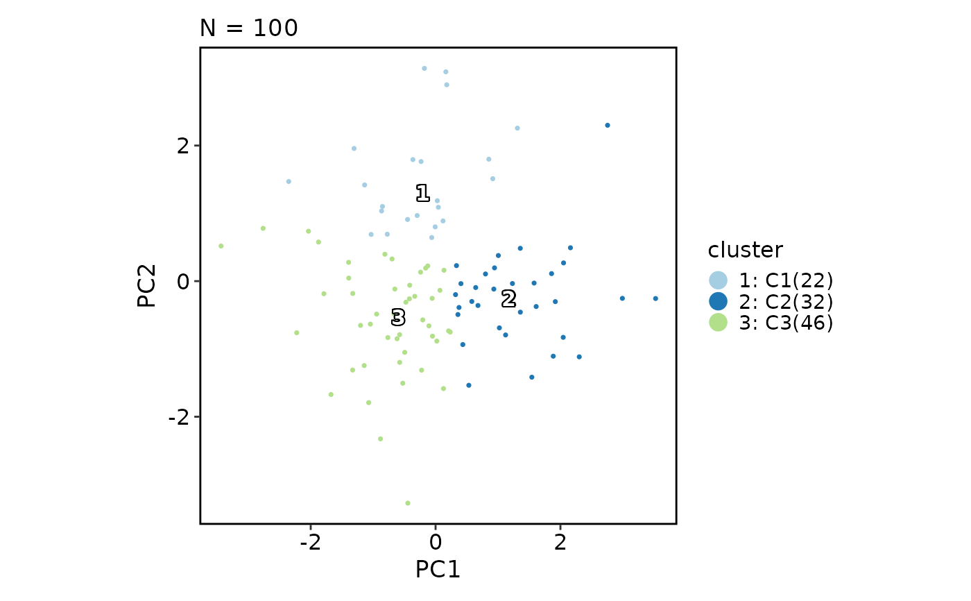
DimPlot(dim_example, group_by = "clusters", label = TRUE,
label_size = 5, label_bg_r = 0.2)
# labels
DimPlot(dim_example, group_by = "clusters", label = TRUE,
label_size = 5, label_bg_r = 0.2)
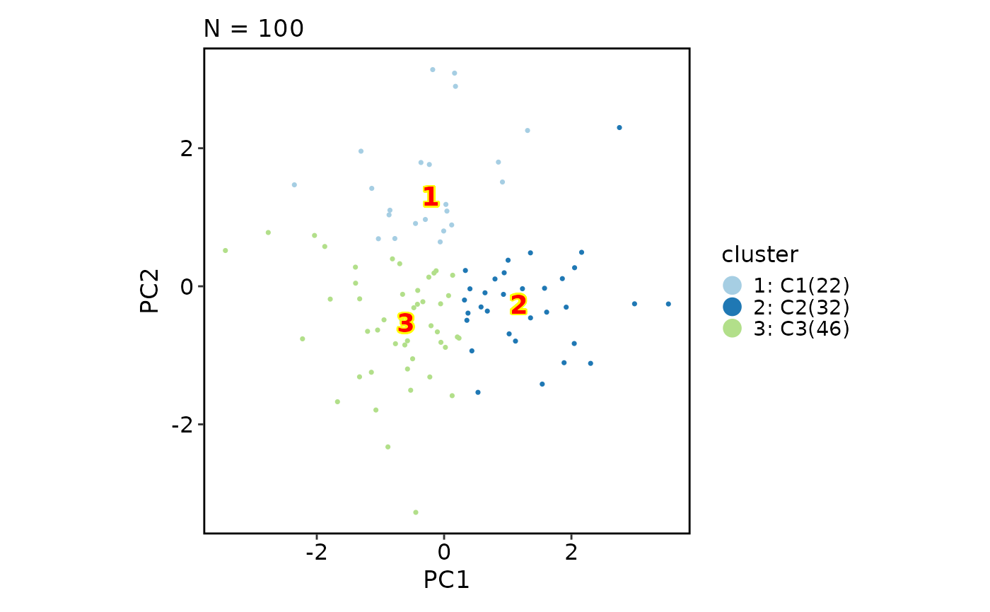
 DimPlot(dim_example, group_by = "clusters", label = TRUE, label_fg = "red",
label_bg = "yellow", label_size = 5)
DimPlot(dim_example, group_by = "clusters", label = TRUE, label_fg = "red",
label_bg = "yellow", label_size = 5)
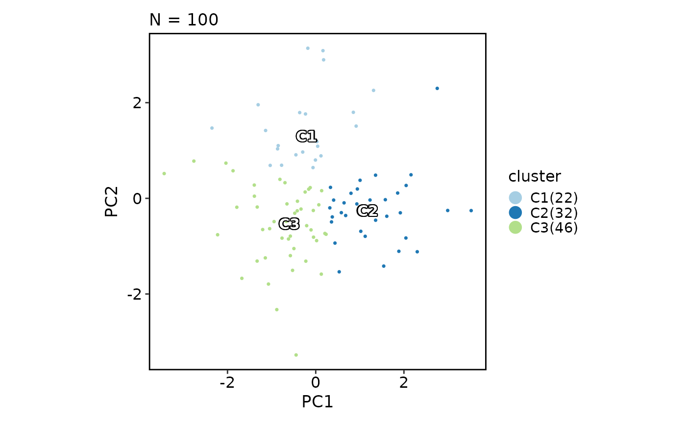
 DimPlot(dim_example, group_by = "clusters", label = TRUE, label_insitu = TRUE)
 # group marks
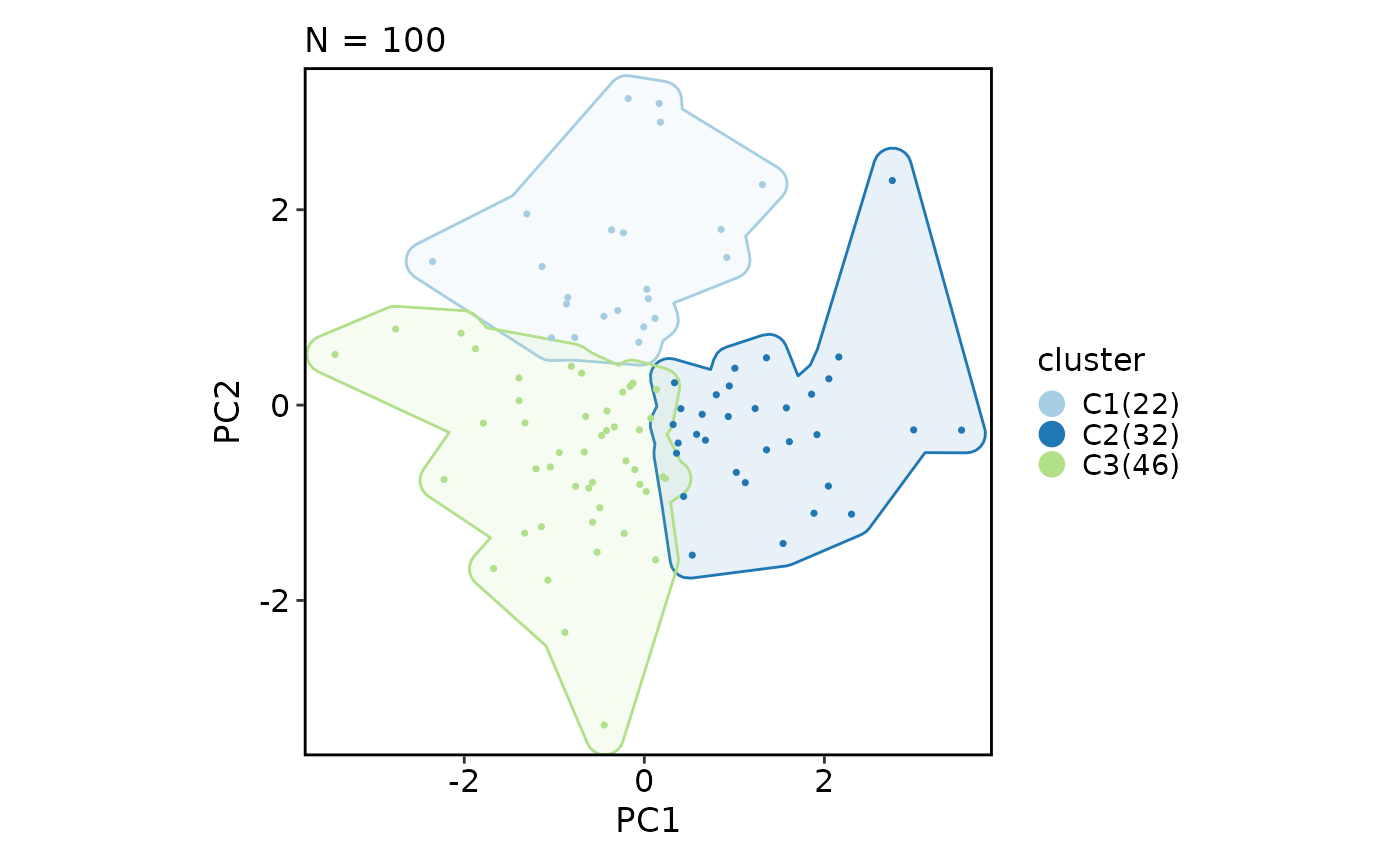
DimPlot(dim_example, group_by = "clusters", add_mark = TRUE)
# group marks
DimPlot(dim_example, group_by = "clusters", add_mark = TRUE)
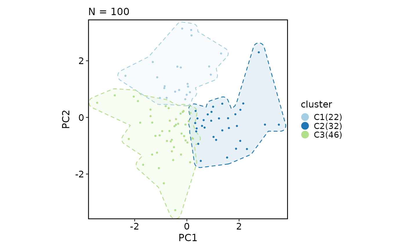
 DimPlot(dim_example, group_by = "clusters", add_mark = TRUE, mark_linetype = 2)
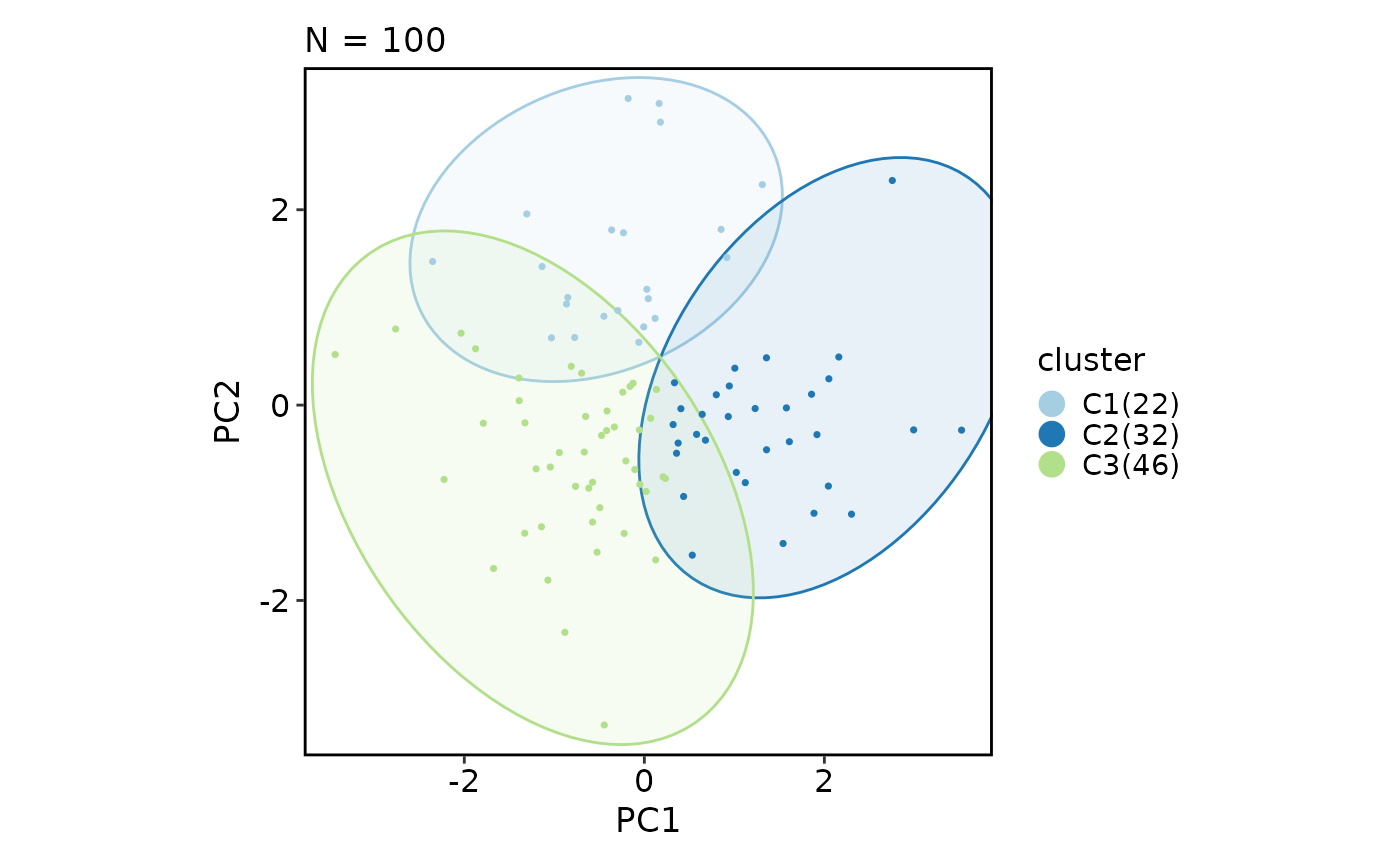
 DimPlot(dim_example, group_by = "clusters", add_mark = TRUE, mark_type = "ellipse")
 # density overlays
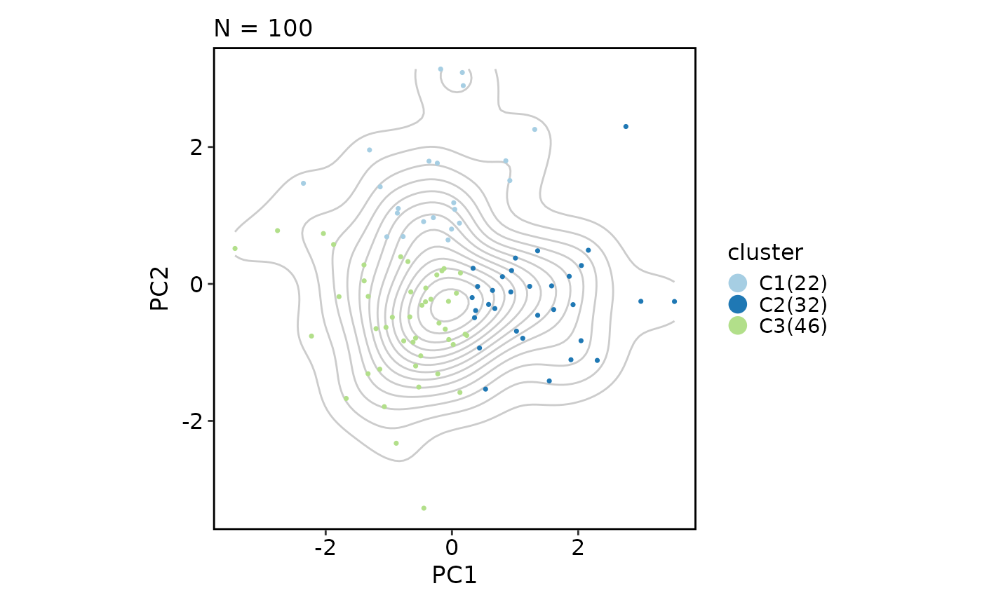
DimPlot(dim_example, group_by = "clusters", add_density = TRUE)
# density overlays
DimPlot(dim_example, group_by = "clusters", add_density = TRUE)
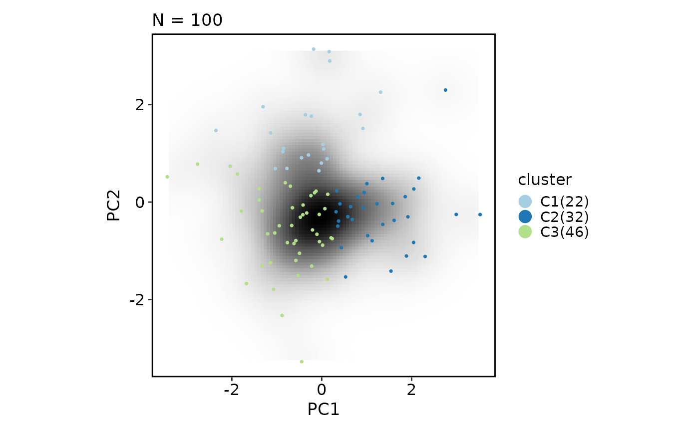
 DimPlot(dim_example, group_by = "clusters", add_density = TRUE, density_filled = TRUE)
#> Warning: Removed 396 rows containing missing values or values outside the scale range
#> (`geom_raster()`).
DimPlot(dim_example, group_by = "clusters", add_density = TRUE, density_filled = TRUE)
#> Warning: Removed 396 rows containing missing values or values outside the scale range
#> (`geom_raster()`).
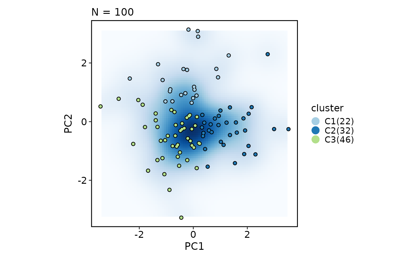
 DimPlot(dim_example, group_by = "clusters", add_density = TRUE, density_filled = TRUE,
density_filled_palette = "Blues", highlight = TRUE)
#> Warning: Removed 396 rows containing missing values or values outside the scale range
#> (`geom_raster()`).
DimPlot(dim_example, group_by = "clusters", add_density = TRUE, density_filled = TRUE,
density_filled_palette = "Blues", highlight = TRUE)
#> Warning: Removed 396 rows containing missing values or values outside the scale range
#> (`geom_raster()`).
 # statistics at group centroids
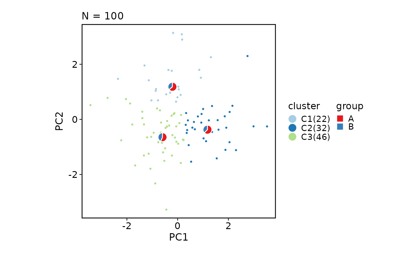
DimPlot(dim_example, group_by = "clusters", stat_by = "group")
# statistics at group centroids
DimPlot(dim_example, group_by = "clusters", stat_by = "group")
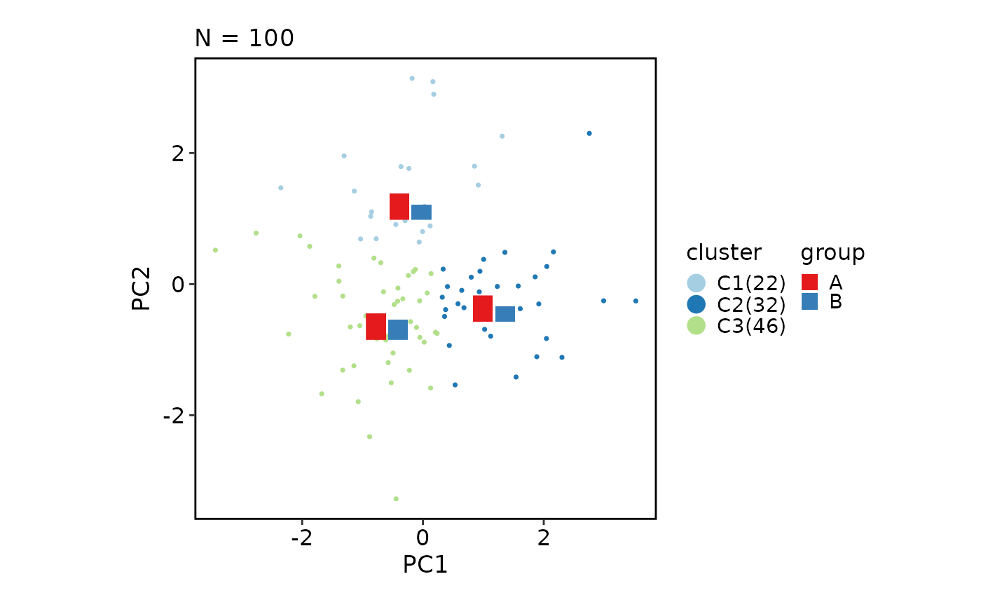
 DimPlot(dim_example, group_by = "clusters", stat_by = "group",
stat_plot_type = "bar", stat_plot_size = 0.06)
DimPlot(dim_example, group_by = "clusters", stat_by = "group",
stat_plot_type = "bar", stat_plot_size = 0.06)
 # hex bins
DimPlot(dim_example, group_by = "clusters", hex = TRUE)
#> Warning: Removed 1 row containing missing values or values outside the scale range
#> (`geom_hex()`).
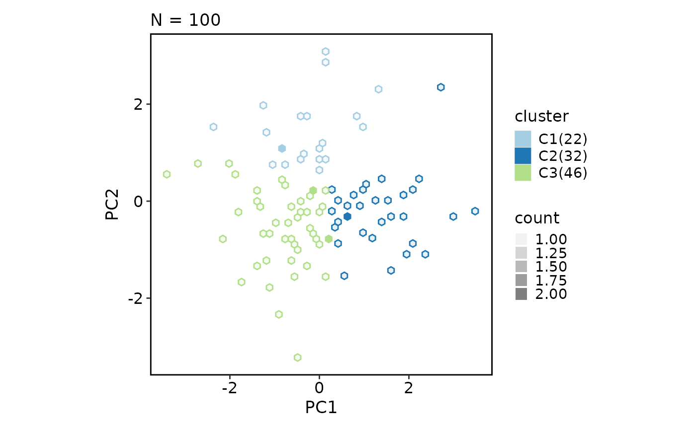
# hex bins
DimPlot(dim_example, group_by = "clusters", hex = TRUE)
#> Warning: Removed 1 row containing missing values or values outside the scale range
#> (`geom_hex()`).
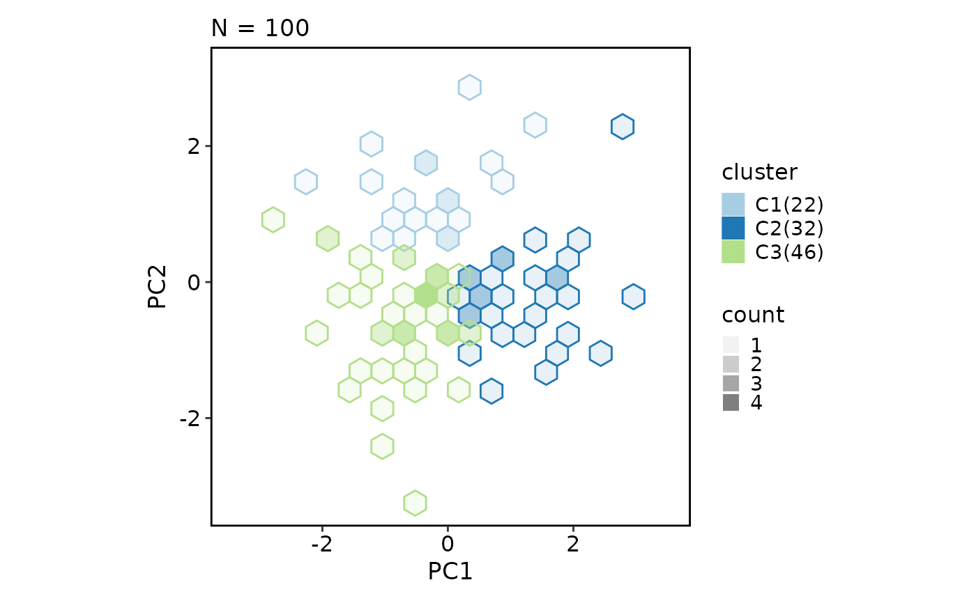
 DimPlot(dim_example, group_by = "clusters", hex = TRUE, hex_bins = 20)
#> Warning: Removed 5 rows containing missing values or values outside the scale range
#> (`geom_hex()`).
DimPlot(dim_example, group_by = "clusters", hex = TRUE, hex_bins = 20)
#> Warning: Removed 5 rows containing missing values or values outside the scale range
#> (`geom_hex()`).
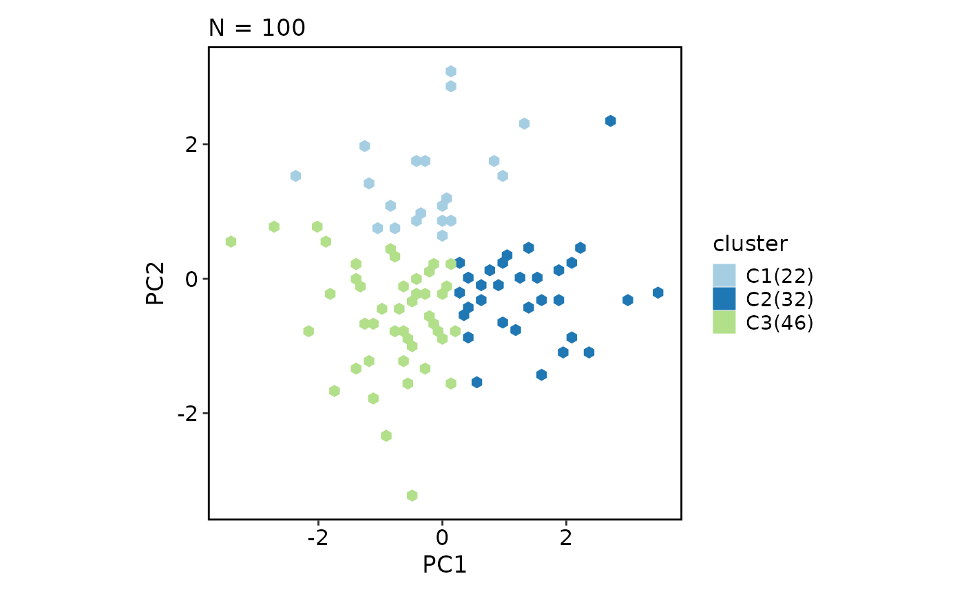
 DimPlot(dim_example, group_by = "clusters", hex = TRUE, hex_count = FALSE)
#> Warning: Removed 1 row containing missing values or values outside the scale range
#> (`geom_hex()`).
DimPlot(dim_example, group_by = "clusters", hex = TRUE, hex_count = FALSE)
#> Warning: Removed 1 row containing missing values or values outside the scale range
#> (`geom_hex()`).
 # graph / network edges
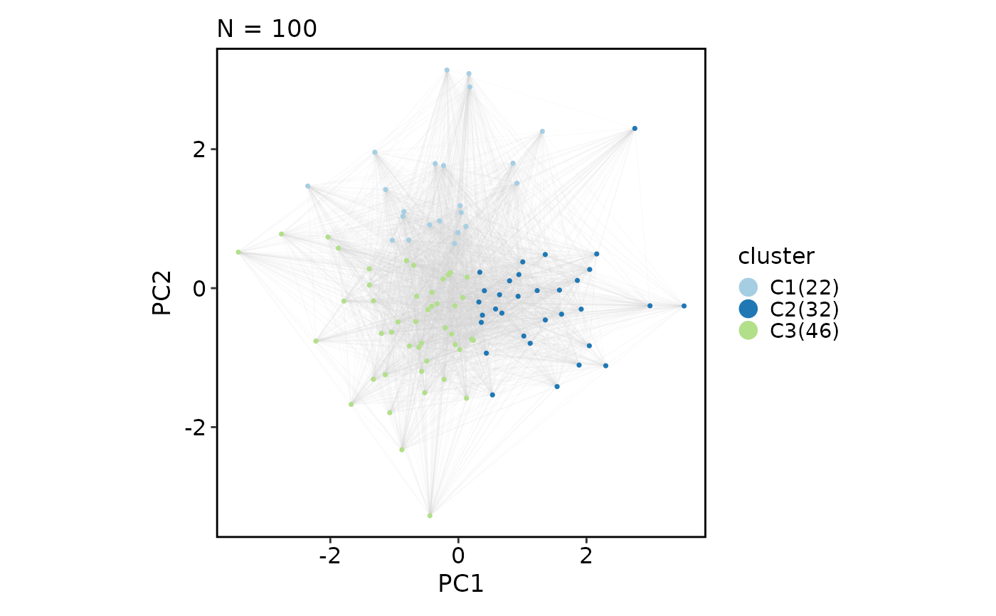
DimPlot(dim_example, group_by = "clusters", graph = "@graph", edge_color = "grey80")
# graph / network edges
DimPlot(dim_example, group_by = "clusters", graph = "@graph", edge_color = "grey80")
 # lineages / trajectories
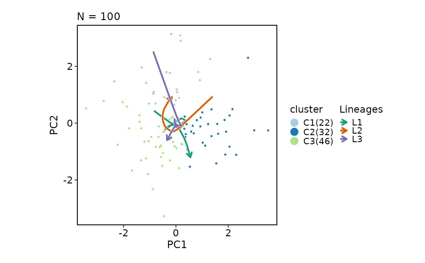
DimPlot(dim_example, group_by = "clusters", lineages = c("stochasticbasis_1", "stochasticbasis_2"))
# lineages / trajectories
DimPlot(dim_example, group_by = "clusters", lineages = c("stochasticbasis_1", "stochasticbasis_2"))
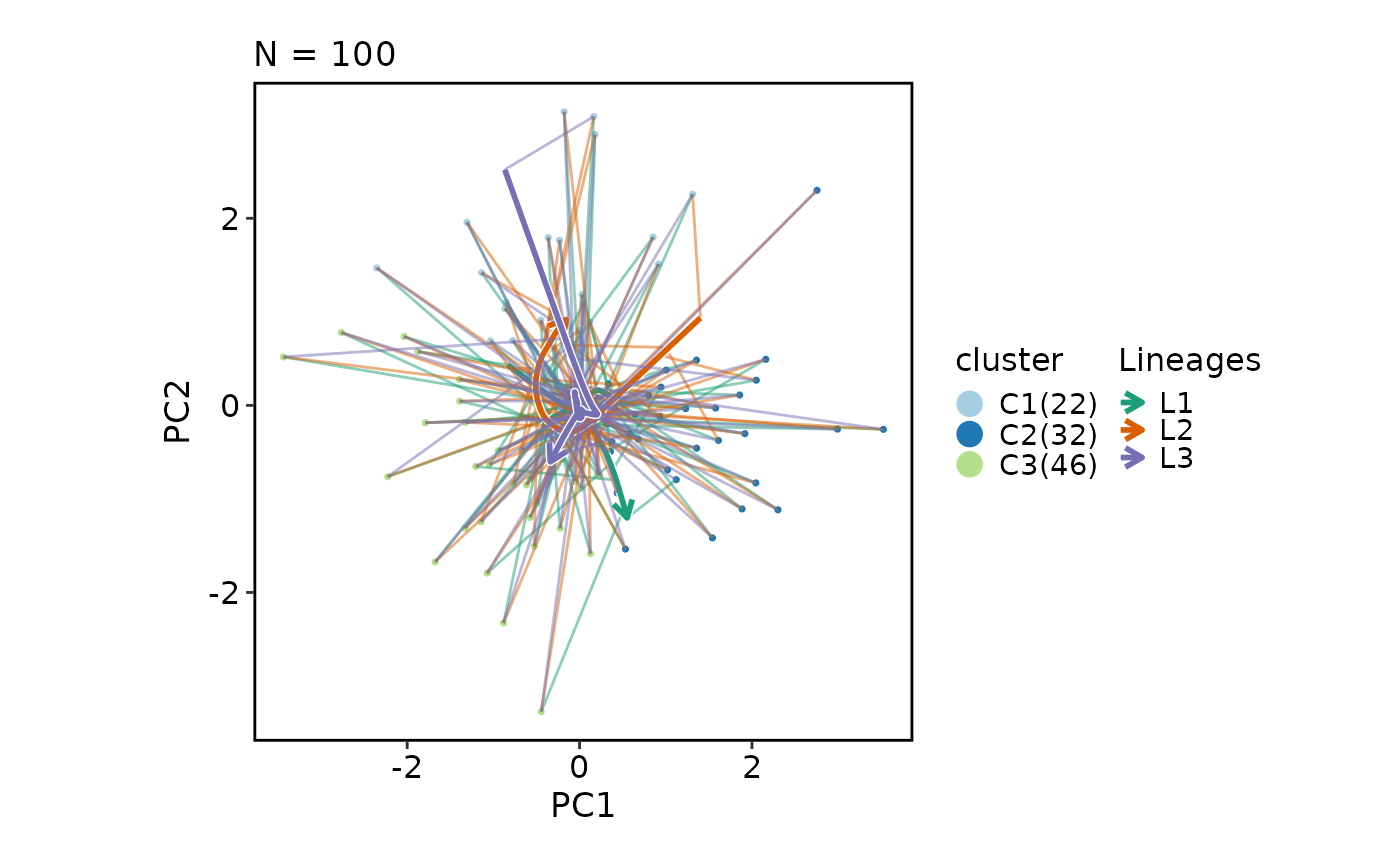
 DimPlot(dim_example, group_by = "clusters", lineages = c("stochasticbasis_1", "stochasticbasis_2"),
lineages_whiskers = TRUE, lineages_whiskers_linewidth = 0.1)
DimPlot(dim_example, group_by = "clusters", lineages = c("stochasticbasis_1", "stochasticbasis_2"),
lineages_whiskers = TRUE, lineages_whiskers_linewidth = 0.1)
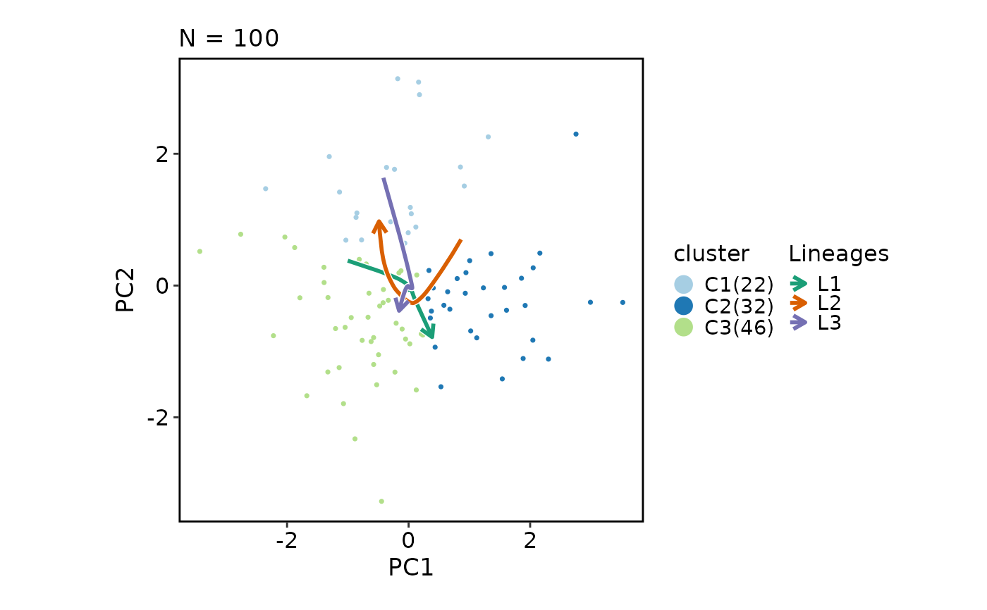
 DimPlot(dim_example, group_by = "clusters", lineages = c("stochasticbasis_1", "stochasticbasis_2"),
lineages_span = 0.4)
DimPlot(dim_example, group_by = "clusters", lineages = c("stochasticbasis_1", "stochasticbasis_2"),
lineages_span = 0.4)
 # split_by
DimPlot(dim_example, group_by = "clusters", split_by = "group",
palette = list(A = "Paired", B = "Set1"))
# split_by
DimPlot(dim_example, group_by = "clusters", split_by = "group",
palette = list(A = "Paired", B = "Set1"))
 # velocity
DimPlot(dim_example, group_by = "clusters", velocity = c("stochasticbasis_1", "stochasticbasis_2"),
pt_alpha = 0)
#> Warning: Removed 1 row containing missing values or values outside the scale range
#> (`geom_segment()`).
# velocity
DimPlot(dim_example, group_by = "clusters", velocity = c("stochasticbasis_1", "stochasticbasis_2"),
pt_alpha = 0)
#> Warning: Removed 1 row containing missing values or values outside the scale range
#> (`geom_segment()`).
 DimPlot(dim_example, group_by = "clusters", velocity = 3:4,
velocity_plot_type = "grid", arrow_alpha = 0.6)
#> Warning: Removed 6 rows containing missing values or values outside the scale range
#> (`geom_segment()`).
DimPlot(dim_example, group_by = "clusters", velocity = 3:4,
velocity_plot_type = "grid", arrow_alpha = 0.6)
#> Warning: Removed 6 rows containing missing values or values outside the scale range
#> (`geom_segment()`).
 DimPlot(dim_example, group_by = "clusters", velocity = 3:4,
velocity_plot_type = "stream")
DimPlot(dim_example, group_by = "clusters", velocity = 3:4,
velocity_plot_type = "stream")
 # 3D plots (returns a plotly object)
DimPlot(dim_example, dims = 1:3, group_by = "clusters")
DimPlot(dim_example, dims = 1:3, group_by = "clusters", label = TRUE,
label_insitu = TRUE)
DimPlot(dim_example, dims = c("basis_1", "basis_2", "stochasticbasis_1"),
group_by = "clusters", graph = "@graph", edge_color = "grey80")
# keep_na and keep_empty
dim_example$clusters[dim_example$clusters == "Ductal"] <- NA
DimPlot(dim_example, group_by = "clusters", keep_na = FALSE, keep_empty = TRUE)
# 3D plots (returns a plotly object)
DimPlot(dim_example, dims = 1:3, group_by = "clusters")
DimPlot(dim_example, dims = 1:3, group_by = "clusters", label = TRUE,
label_insitu = TRUE)
DimPlot(dim_example, dims = c("basis_1", "basis_2", "stochasticbasis_1"),
group_by = "clusters", graph = "@graph", edge_color = "grey80")
# keep_na and keep_empty
dim_example$clusters[dim_example$clusters == "Ductal"] <- NA
DimPlot(dim_example, group_by = "clusters", keep_na = FALSE, keep_empty = TRUE)
 DimPlot(dim_example, group_by = "clusters", keep_na = TRUE, keep_empty = TRUE)
 DimPlot(dim_example, group_by = "clusters", keep_na = TRUE, keep_empty = FALSE)
 # }
# \donttest{
data(dim_example)
# single feature
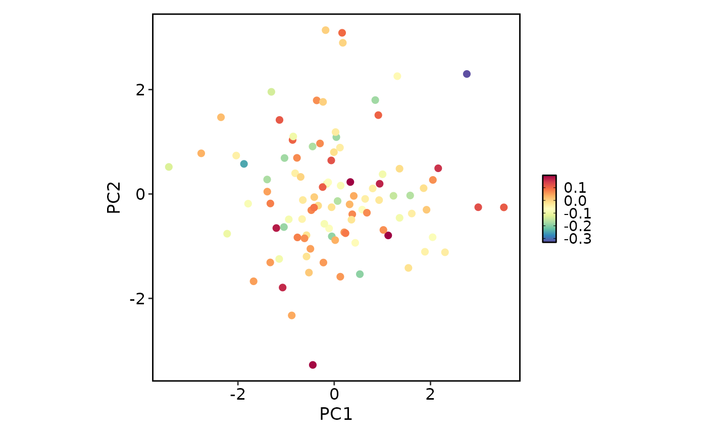
FeatureDimPlot(dim_example, features = "stochasticbasis_1", pt_size = 2)
# }
# \donttest{
data(dim_example)
# single feature
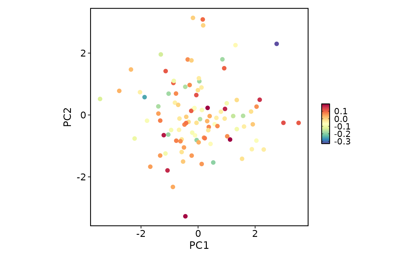
FeatureDimPlot(dim_example, features = "stochasticbasis_1", pt_size = 2)
 FeatureDimPlot(dim_example, features = "stochasticbasis_1", pt_size = 2, bg_cutoff = 0)
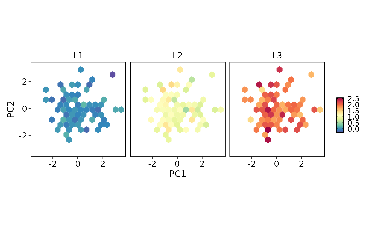 FeatureDimPlot(dim_example, features = "stochasticbasis_1", raster = TRUE, raster_dpi = 30)
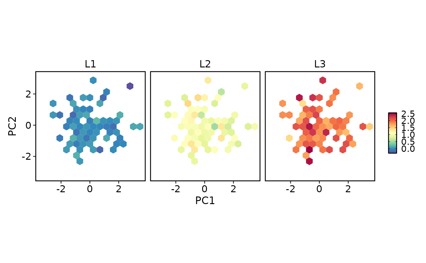 # multiple features (auto-pivoted to long, faceted by feature)
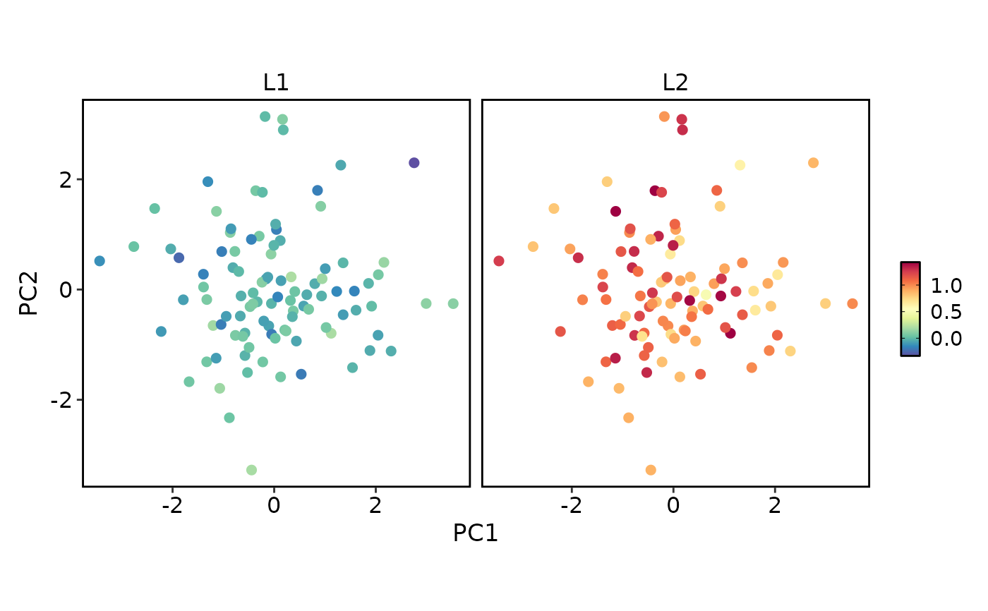
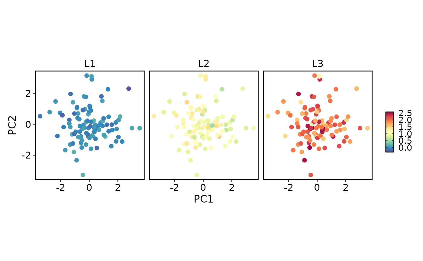
FeatureDimPlot(dim_example, features = c("stochasticbasis_1", "stochasticbasis_2"),
pt_size = 2)
# multiple features (auto-pivoted to long, faceted by feature)
FeatureDimPlot(dim_example, features = c("stochasticbasis_1", "stochasticbasis_2"),
pt_size = 2)
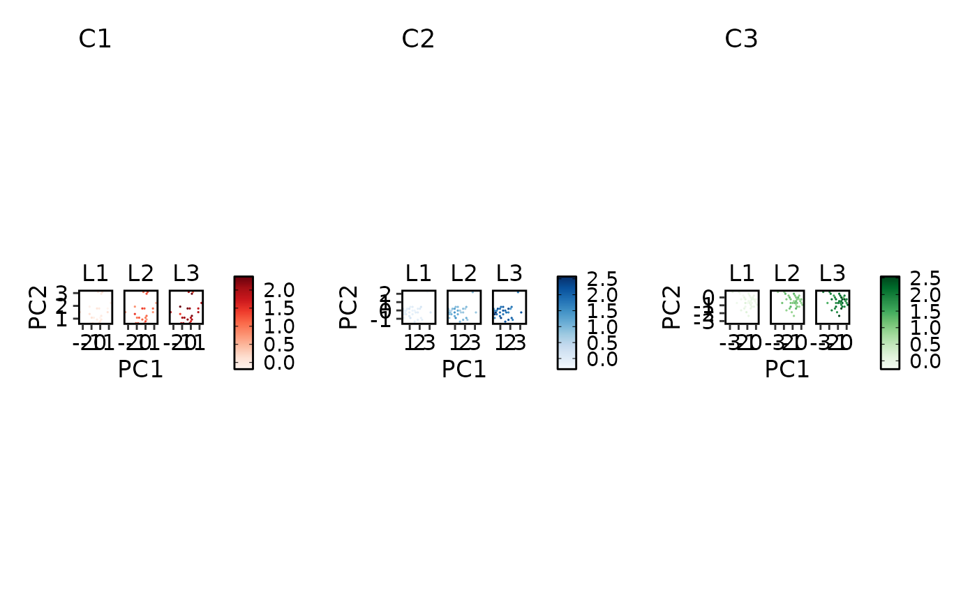 # single feature with facet_by (facet_by works when only 1 feature)
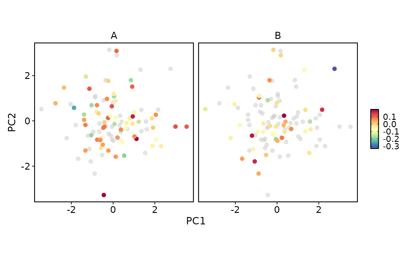
FeatureDimPlot(dim_example, features = c("stochasticbasis_1"), pt_size = 2,
facet_by = "group")
# single feature with facet_by (facet_by works when only 1 feature)
FeatureDimPlot(dim_example, features = c("stochasticbasis_1"), pt_size = 2,
facet_by = "group")
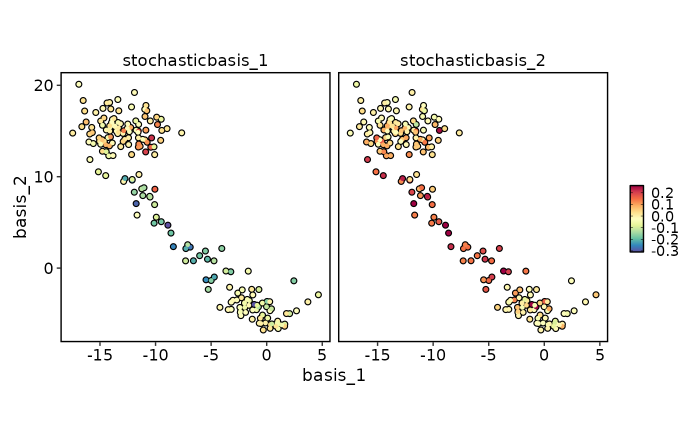 # multiple features with split_by for independent layout
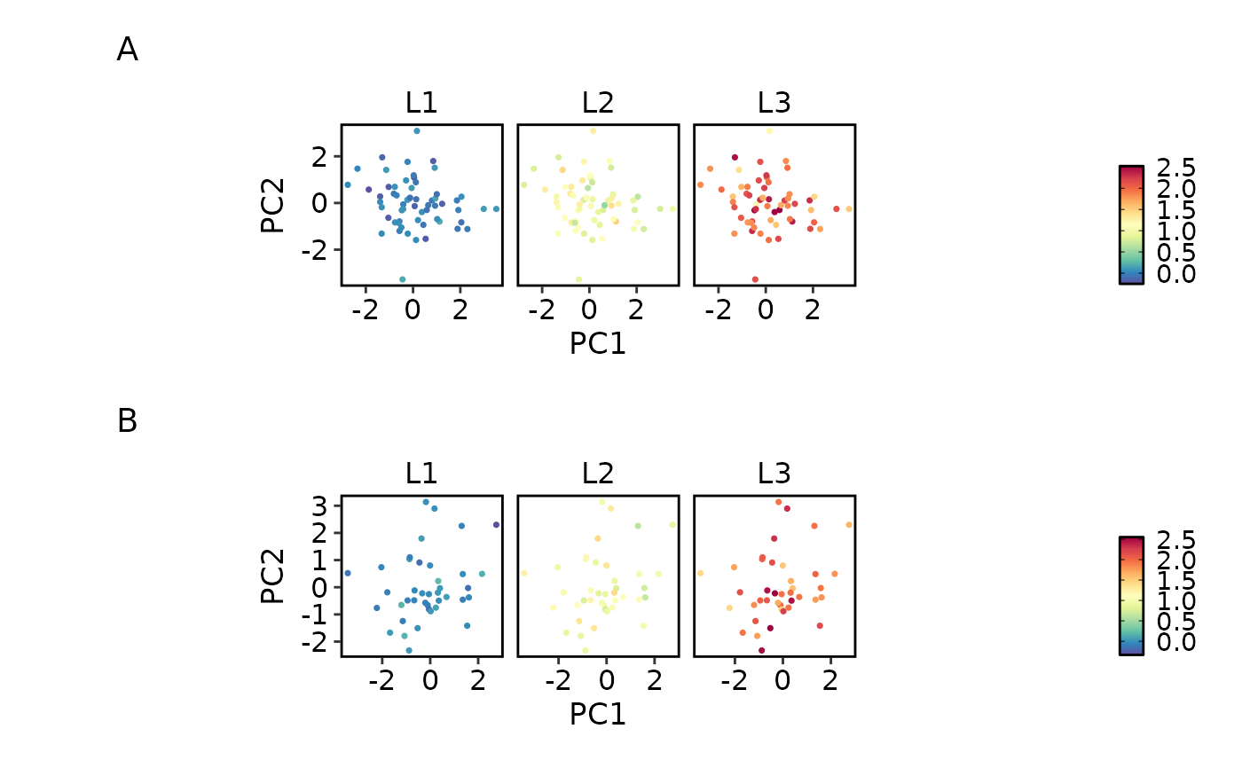
FeatureDimPlot(dim_example, features = c("stochasticbasis_1", "stochasticbasis_2"),
split_by = "group", nrow = 2)
# multiple features with split_by for independent layout
FeatureDimPlot(dim_example, features = c("stochasticbasis_1", "stochasticbasis_2"),
split_by = "group", nrow = 2)
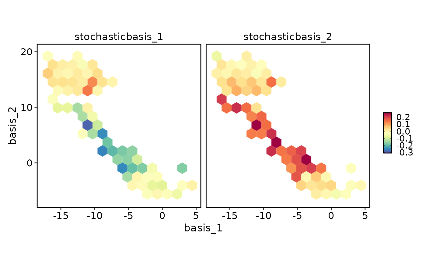 # highlight and hex
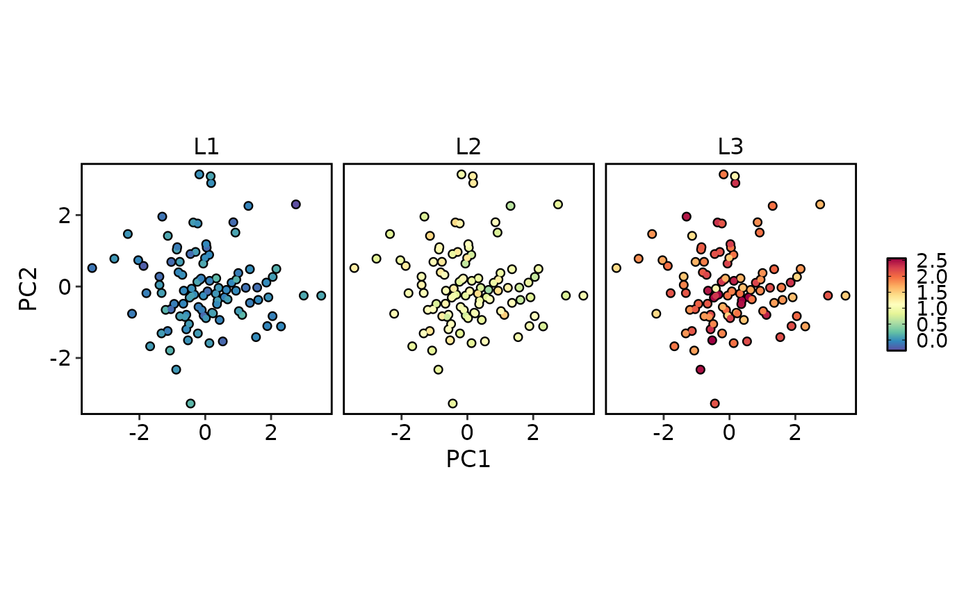
FeatureDimPlot(dim_example, features = c("stochasticbasis_1", "stochasticbasis_2"),
highlight = TRUE)
# highlight and hex
FeatureDimPlot(dim_example, features = c("stochasticbasis_1", "stochasticbasis_2"),
highlight = TRUE)
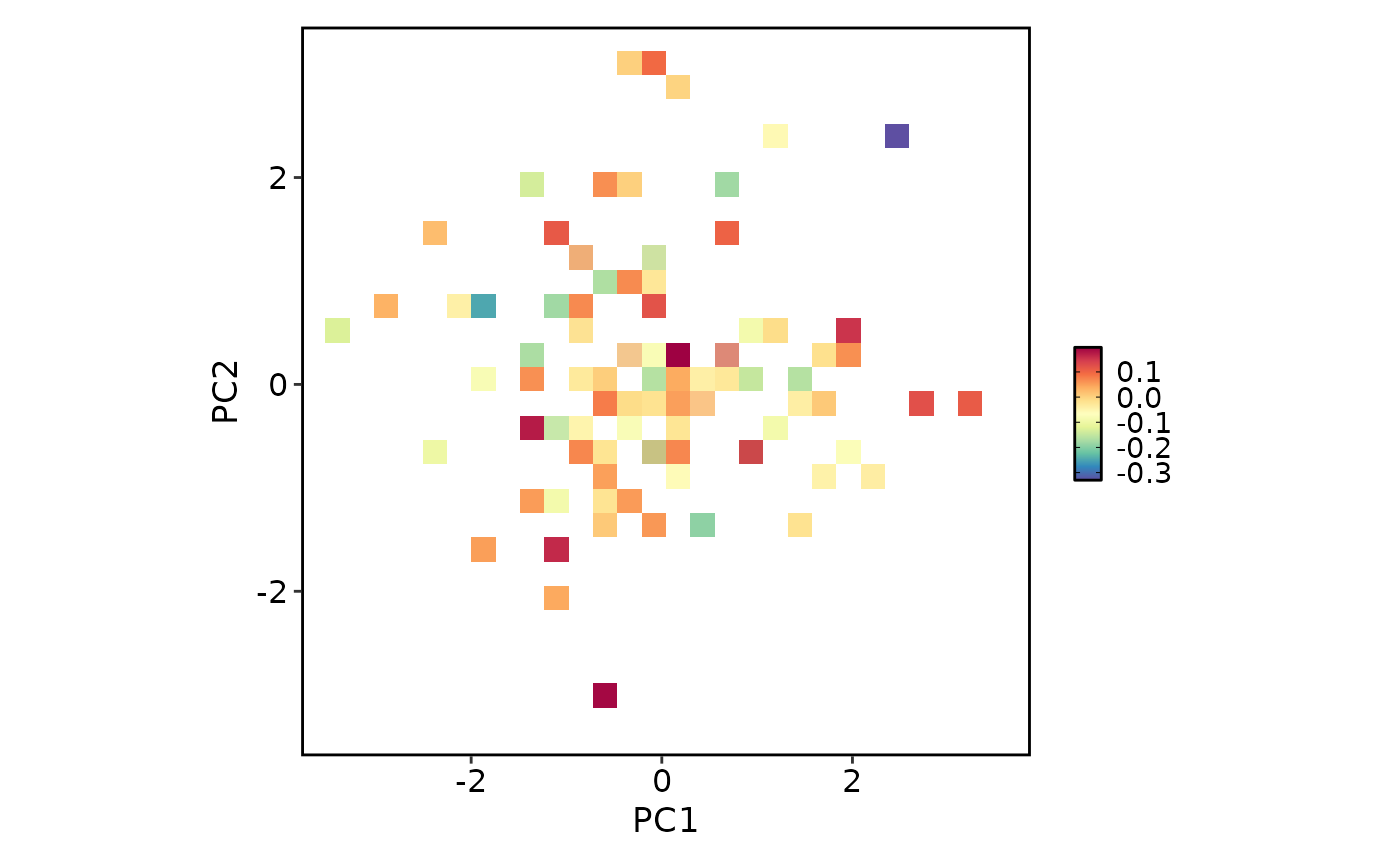
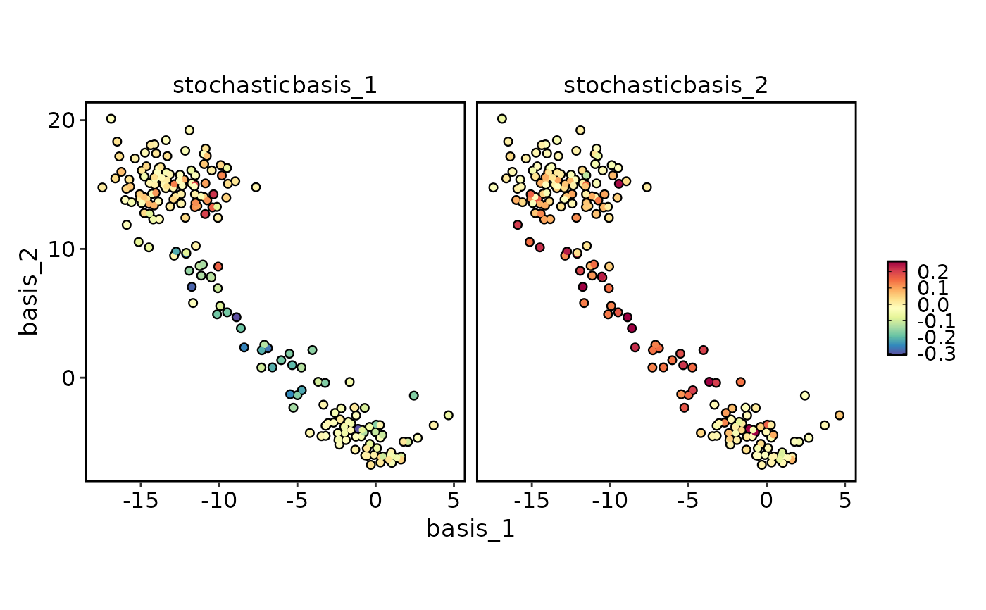
 FeatureDimPlot(dim_example, features = c("stochasticbasis_1", "stochasticbasis_2"),
hex = TRUE, hex_bins = 15)
#> Warning: Removed 8 rows containing missing values or values outside the scale range
#> (`geom_hex()`).
FeatureDimPlot(dim_example, features = c("stochasticbasis_1", "stochasticbasis_2"),
hex = TRUE, hex_bins = 15)
#> Warning: Removed 8 rows containing missing values or values outside the scale range
#> (`geom_hex()`).
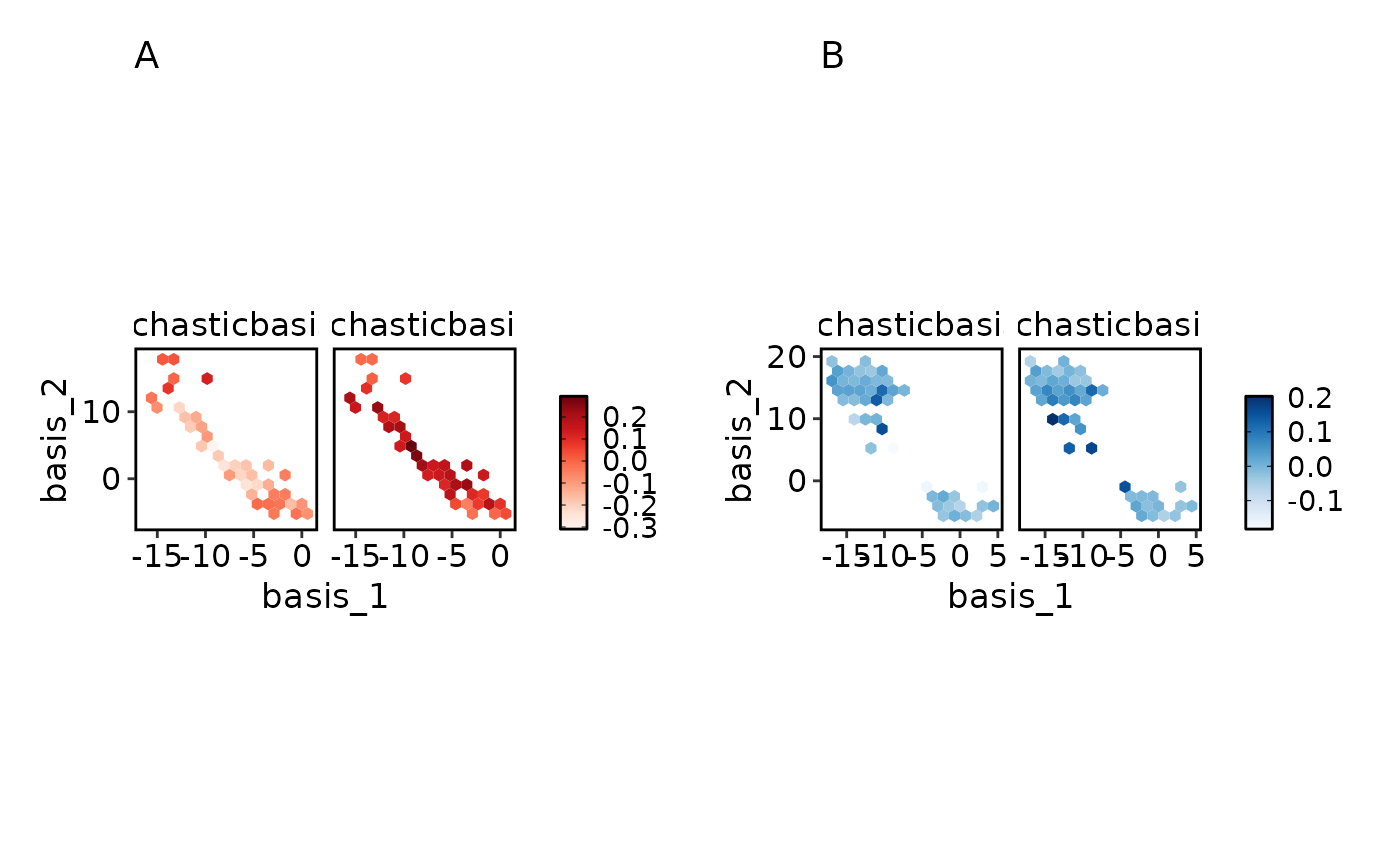
 FeatureDimPlot(dim_example, features = c("stochasticbasis_1", "stochasticbasis_2"),
hex = TRUE, hex_bins = 15, split_by = "group", palette = list(A = "Reds", B = "Blues"))
#> Warning: Removed 6 rows containing missing values or values outside the scale range
#> (`geom_hex()`).
#> Warning: Removed 8 rows containing missing values or values outside the scale range
#> (`geom_hex()`).
FeatureDimPlot(dim_example, features = c("stochasticbasis_1", "stochasticbasis_2"),
hex = TRUE, hex_bins = 15, split_by = "group", palette = list(A = "Reds", B = "Blues"))
#> Warning: Removed 6 rows containing missing values or values outside the scale range
#> (`geom_hex()`).
#> Warning: Removed 8 rows containing missing values or values outside the scale range
#> (`geom_hex()`).
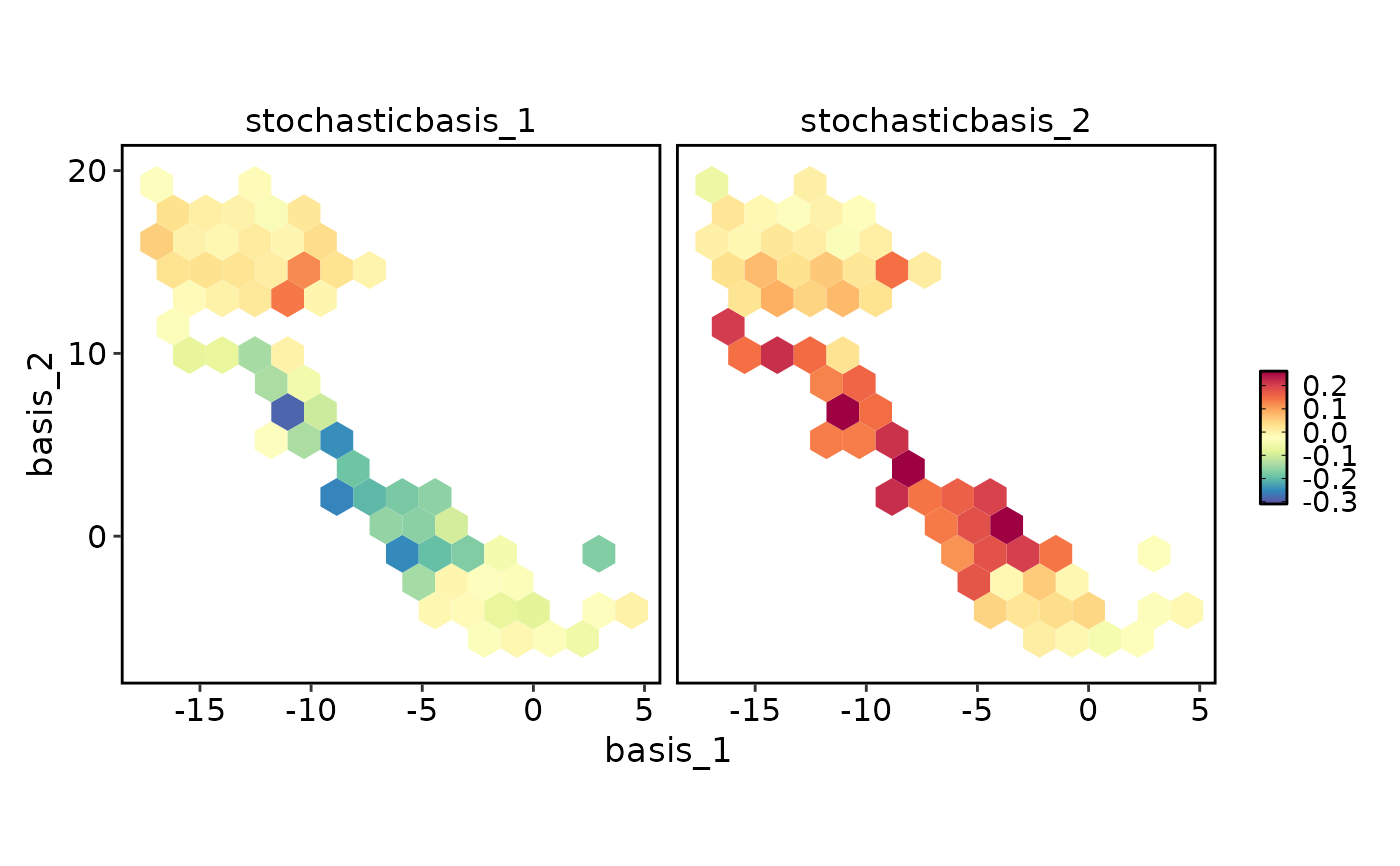 # 3D plots (returns a plotly object)
FeatureDimPlot(dim_example, dims = 1:3, features = "stochasticbasis_2", pt_size = 2)
FeatureDimPlot(dim_example, dims = c("basis_1", "basis_2", "stochasticbasis_1"),
features = "stochasticbasis_2")
# }
# 3D plots (returns a plotly object)
FeatureDimPlot(dim_example, dims = 1:3, features = "stochasticbasis_2", pt_size = 2)
FeatureDimPlot(dim_example, dims = c("basis_1", "basis_2", "stochasticbasis_1"),
features = "stochasticbasis_2")
# }