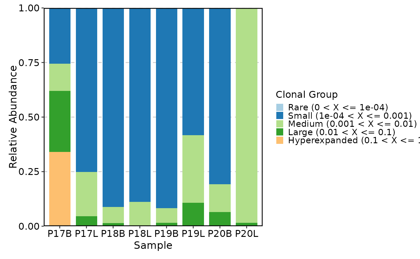
Clonal Composition Plot — ClonalCompositionPlot • scplotter

Visualizes the composition of the immune repertoire by categorizing clones into abundance groups (Rare, Small, Medium, Large, Hyperexpanded) and plotting their relative proportions across samples or metadata groups. This reveals the overall structure of the repertoire — whether it is dominated by a few large clones (clonal expansion) or composed of many small clones (high diversity).

ClonalCompositionPlot supports three analysis methods:

Homeostasis ("homeostasis", "homeo", "rel") — Clones are binned by their frequency (fraction of the total repertoire) into categories such as Rare, Small, Medium, Large, and Hyperexpanded. Uses scRepertoire::clonalHomeostasis().
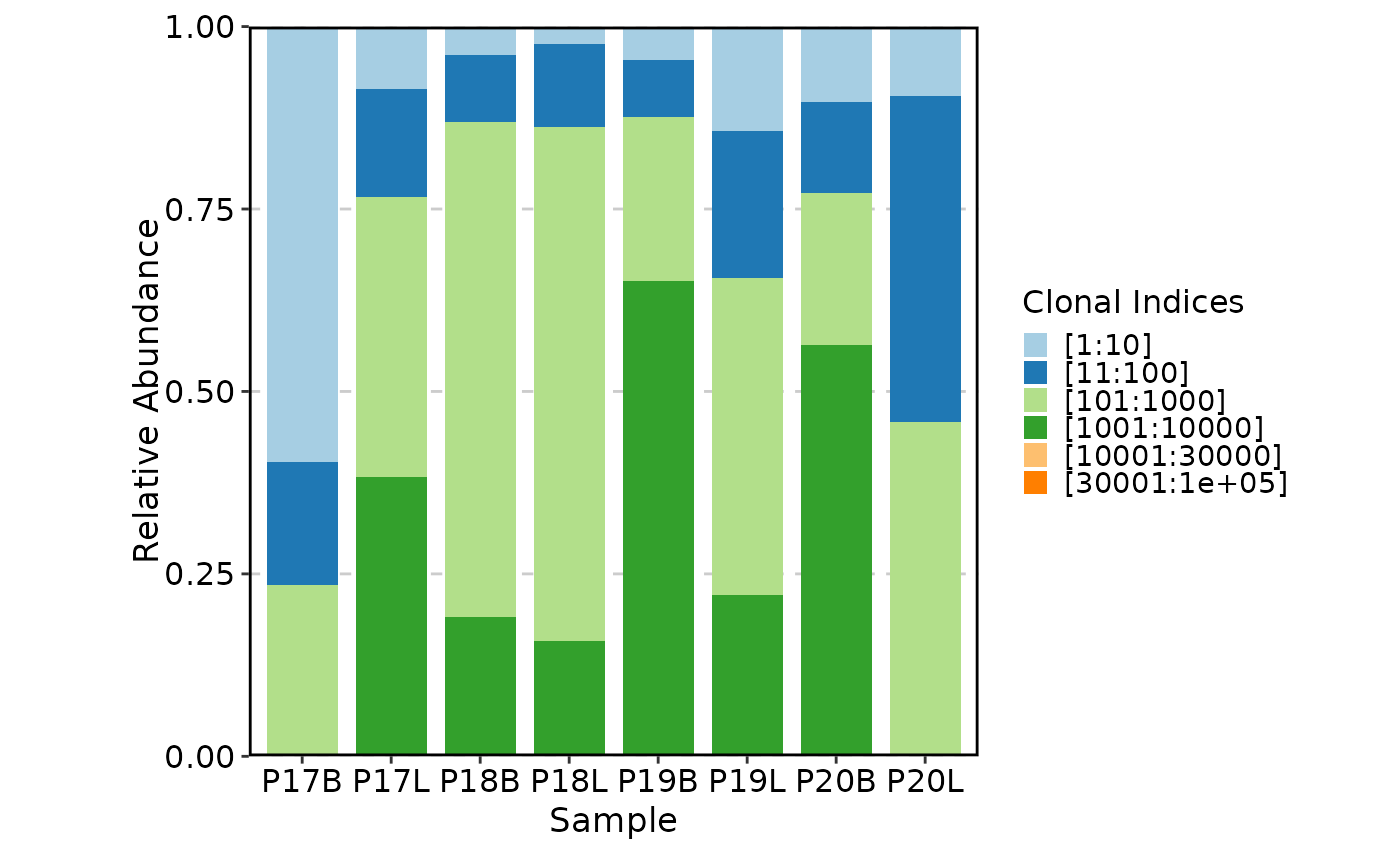
Top clones ("top") — Clones are ranked and binned by their rank index (e.g., top 10, top 100, etc.). Uses scRepertoire::clonalProportion().
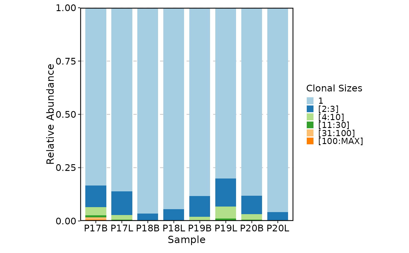
Rare clones ("rare") — Clones are binned by their absolute size (clone count). Uses clone size thresholds directly.

Usage

ClonalCompositionPlot(
  data,
  clone_call = "aa",
  chain = "both",
  method = c("homeostasis", "homeo", "rel", "top", "rare"),
  clone_split = NULL,
  scale = TRUE,
  facet_by = NULL,
  group_by = NULL,
  split_by = NULL,
  xlab = NULL,
  ylab = NULL,
  plot_type = c("bar", "ring", "box", "violin"),
  order = NULL,
  ...
)

Arguments

data

The product of scRepertoire::combineTCR(), scRepertoire::combineBCR(), or scRepertoire::combineExpression().

clone_call

How to define a clone. One of "gene", "nt", "aa" (default), "strict", or a custom variable name in the data.

chain

Which chain(s) to use: "both" (default), "TRA", "TRB", "TRD", "TRG", "IGH", or "IGL".

method

The clonal categorization method. One of:

"homeostasis" (default), "homeo", "rel" — Frequency-based binning using clone_split as abundance thresholds.
"top" — Rank-based binning using clone_split as rank cutoffs.
"rare" — Size-based binning using clone_split as clone size thresholds.

clone_split

Threshold values defining the clonal categories. Default is NULL, which picks sensible defaults per method:

For "homeostasis"/"homeo"/"rel" — a named list of frequency thresholds: list(Rare = 1e-04, Small = 0.001, Medium = 0.01, Large = 0.1, Hyperexpanded = 1)
For "top" — rank cutoffs: c(10, 100, 1000, 10000, 30000, 100000)
For "rare" — clone size thresholds: c(1, 3, 10, 30, 100)

scale

How to normalize the values. One of:

TRUE (default) — Values within each x-axis group sum to 1 (group-wise proportion).
FALSE — Raw values (clone counts) are used.
"sample" or "Sample" — Values within each sample sum to 1 (sample-wise proportion).

facet_by

Metadata column used to facet the plot into separate panels. Default is NULL.

group_by

Metadata column used to group (color) the data. Default is NULL. Required for "box" and "violin" plot types.

split_by

Metadata column used to split the data into separate plots. Default is NULL.

xlab

X-axis label. Default is NULL, which uses the group_by column name or "Sample".

ylab

Y-axis label. Default is NULL, which auto-generates "Abundance" or "Relative Abundance" depending on scale.

plot_type

The visualization type. One of:

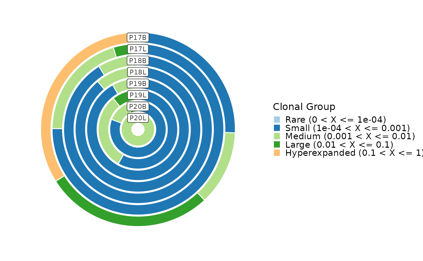
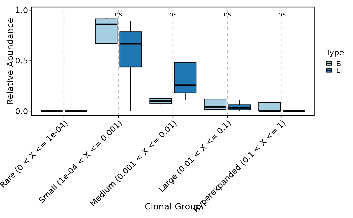
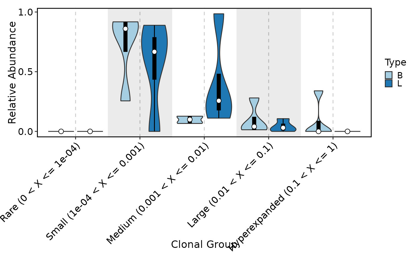
"bar" (default) — Stacked bar chart of clonal categories across groups. Best for comparing composition across categories.
"ring" — Ring (donut) chart alternative to stacked bars.
"box" — Box plot showing the distribution of each clonal category's abundance across samples. Requires group_by.
"violin" — Violin plot alternative to box plot. Requires group_by.

order

A named list controlling the order of factor levels. List names are column names; list values are the desired order. Default is NULL.

...

Additional arguments passed to the underlying plotthis function:

"bar" — plotthis::BarPlot() (palette, position, alpha, ...)
"ring" — plotthis::RingPlot() (palette, alpha, ...)
"box" — plotthis::BoxPlot() (comparisons, add_bg, palette, ...)
"violin" — plotthis::ViolinPlot() (add_box, add_bg, comparisons, palette, ...)

Value

A ggplot object, or a list of ggplot objects if combine = FALSE is passed via ....

Note

group_by for box/violin: The group_by parameter is required when plot_type is "box" or "violin". These plot types show per-sample distributions, with group_by determining the coloring.

Bar/ring aggregation: When group_by is specified for bar or ring plots, data is aggregated across samples within each group (Sample values are summed) before plotting, to show group-level composition.

Examples

# \donttest{
set.seed(8525)
data(contig_list, package = "scRepertoire")
data <- scRepertoire::combineTCR(contig_list,
    samples = c("P17B", "P17L", "P18B", "P18L", "P19B","P19L", "P20B", "P20L"))
data <- scRepertoire::addVariable(data,
    variable.name = "Type",
    variables = factor(rep(c("B", "L"), 4), levels = c("L", "B"))
)
data <- scRepertoire::addVariable(data,
    variable.name = "Subject",
    variables = rep(c("P17", "P18", "P19", "P20"), each = 2)
)

ClonalCompositionPlot(data)

ClonalCompositionPlot(data, method = "top")

ClonalCompositionPlot(data, plot_type = "ring")

ClonalCompositionPlot(data, group_by = "Type", plot_type = "box", comparison = TRUE,
 clone_split = list(Small = 0.001, Medium = 0.01, Large = 0.1, Hyperexpanded = 1))
#> Warning: [Box/Violin/BeeswarmPlot] Some pairwise comparisons may fail due to insufficient data points or variability. Adjusting data to ensure valid comparisons.

ClonalCompositionPlot(data, group_by = "Type", plot_type = "violin", add_box = TRUE,
 add_bg = TRUE)

ClonalCompositionPlot(data, method = "rare")

# }