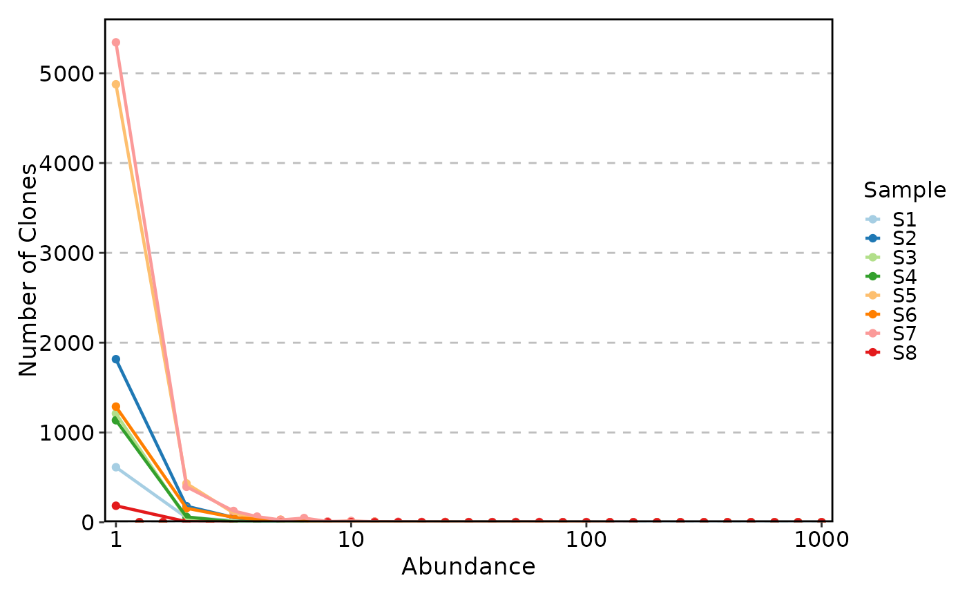
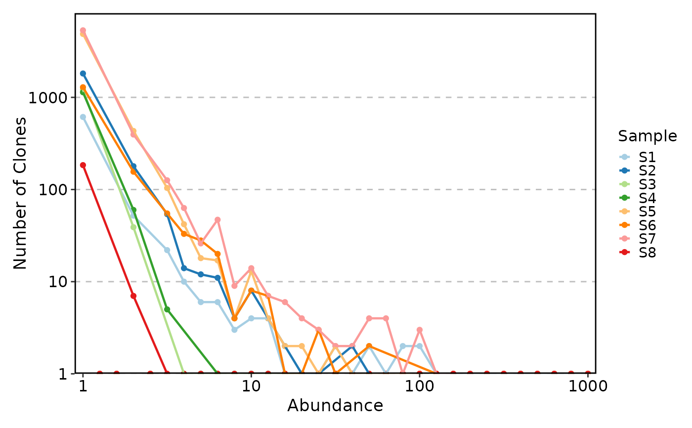
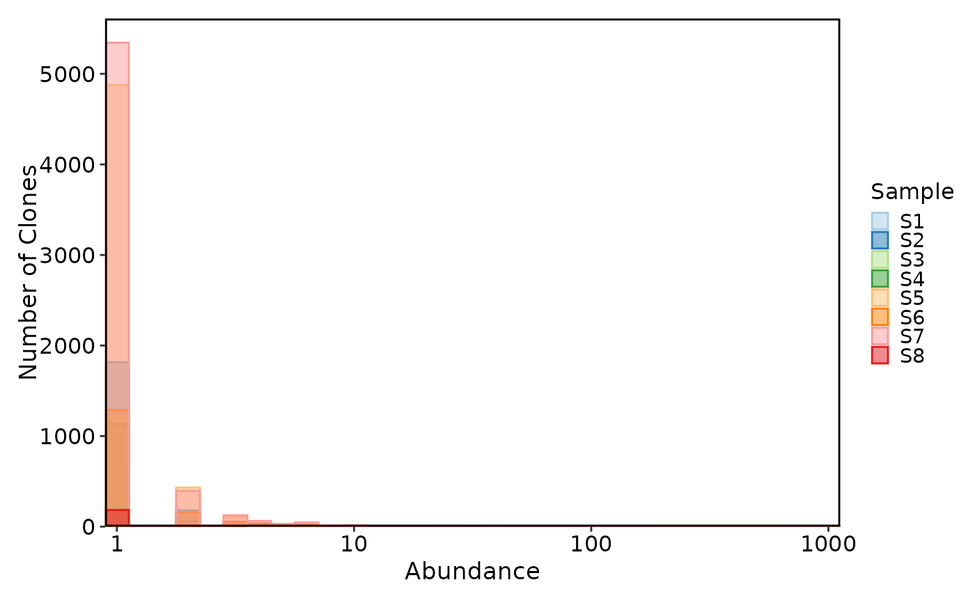
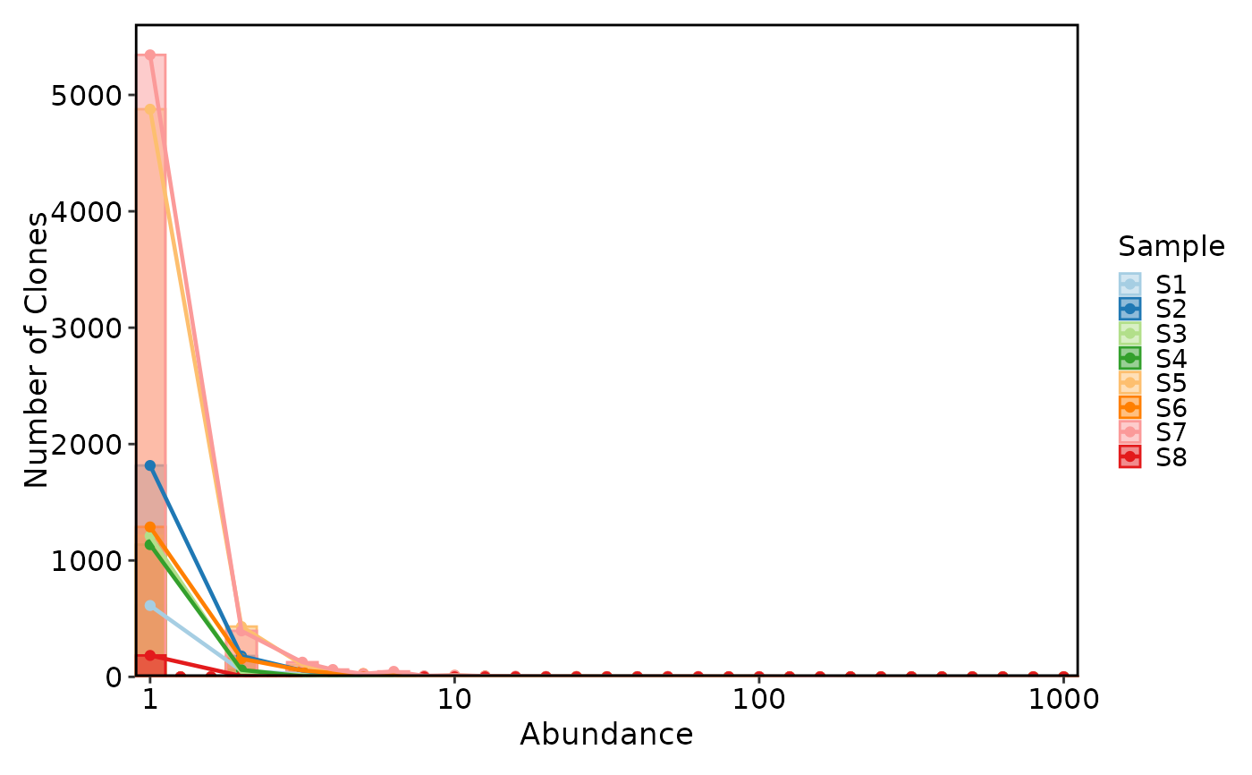
Clonal Abundance Plot — ClonalAbundancePlot • scplotter

Visualizes the distribution of clonal abundances — how many clones are present at each abundance level (frequency) in the repertoire. Clonal abundance distributions typically follow a power-law pattern: a small number of highly expanded clones and a large number of rare clones. This function helps characterize repertoire structure by showing whether the immune response is dominated by a few large clones (clonal expansion) or evenly distributed across many clones (high diversity).

ClonalAbundancePlot computes clonal abundance data via scRepertoire::clonalAbundance() and visualizes it as trend lines, histograms, or density curves.

Usage

ClonalAbundancePlot(
  data,
  clone_call = "aa",
  chain = "both",
  xtrans = "log10",
  ytrans = "identity",
  plot_type = c("trend", "histogram", "density"),
  binwidth = 0.1,
  trend_skip_zero = TRUE,
  bw = 0.5,
  group_by = "Sample",
  group_by_sep = "_",
  facet_by = NULL,
  split_by = NULL,
  order = NULL,
  xlab = "Abundance",
  ylab = NULL,
  theme_args = list(),
  ...
)

Arguments

data

The product of scRepertoire::combineTCR(), scRepertoire::combineBCR(), or scRepertoire::combineExpression().

clone_call

How to define a clone. One of "gene", "nt", "aa" (default), "strict", or a custom variable name in the data.

chain

Which chain(s) to use: "both" (default), "TRA", "TRB", "TRD", "TRG", "IGH", or "IGL".

xtrans

Transformation applied to the x-axis. Default is "log10", which spreads low-abundance clones for better visibility. Use "identity" for linear scale.

ytrans

Transformation applied to the y-axis. Default is "identity". Use "log10" to better visualize distributions spanning multiple orders of magnitude.

plot_type

The visualization type. One of:

"trend" (default) — Smoothed trend line showing the number of clones at each abundance level. The x-axis is transformed by xtrans (default log10), and a LOESS trend is fitted.
"histogram" — Binned histogram of clonal abundances. Optionally overlay a trend line with add_trend = TRUE.
"density" — Kernel density estimate of the abundance distribution.

binwidth

The histogram bin width (in log10-transformed abundance units). Default is 0.1. Only used for "trend" and "histogram" plot types.

trend_skip_zero

Logical; if TRUE (default), zero-abundance bins are excluded from the trend line fit. Improves fit quality when many abundance bins have zero clones.

bw

Smoothing bandwidth for density plots. Higher values produce smoother curves. Default is 0.5.

group_by

Metadata column used to group (color) the data. Default is "Sample".

group_by_sep

Separator used when concatenating multiple group_by columns. Default is "_".

facet_by

Metadata column used to facet the plot into separate panels. Default is NULL.

split_by

Metadata column used to split the data into separate plots. Default is NULL.

order

A named list controlling the order of factor levels. List names are column names; list values are the desired order. Default is NULL.

xlab

X-axis label. Default is "Abundance".

ylab

Y-axis label. Default is NULL, which auto-generates "Number of Clones" (trend/histogram) or "Density of Clones" (density).

theme_args

A list of theme elements passed to the underlying plotthis function. Default is an empty list.

...

Additional arguments passed to the underlying plotthis function:

"trend" — plotthis::Histogram() (with use_trend = TRUE; palette, alpha, ...)
"histogram" — plotthis::Histogram() (add_trend, palette, alpha, ...)
"density" — plotthis::DensityPlot() (palette, alpha, ...)

Value

A ggplot object, or a list of ggplot objects if combine = FALSE is passed via ....

Examples

# \donttest{
set.seed(8525)
data(contig_list, package = "scRepertoire")
data <- scRepertoire::combineTCR(contig_list)
data <- scRepertoire::addVariable(data,
    variable.name = "Type",
    variables = factor(sample(c("B", "L"), 8, replace = TRUE), levels = c("L", "B"))
)
data <- scRepertoire::addVariable(data,
    variable.name = "Sex",
    variables = factor(sample(c("M", "F"), 8, replace = TRUE), levels = c("M", "F"))
)

ClonalAbundancePlot(data)
#> Warning: Removed 104 rows containing missing values or values outside the scale range
#> (`geom_line()`).

ClonalAbundancePlot(data, ytrans = "log10")
#> Warning: log-10 transformation introduced infinite values.
#> Warning: Removed 104 rows containing missing values or values outside the scale range
#> (`geom_line()`).

ClonalAbundancePlot(data, plot_type = "histogram")

ClonalAbundancePlot(data, plot_type = "histogram", add_trend = TRUE, trend_skip_zero = TRUE)
#> Warning: Removed 104 rows containing missing values or values outside the scale range
#> (`geom_line()`).

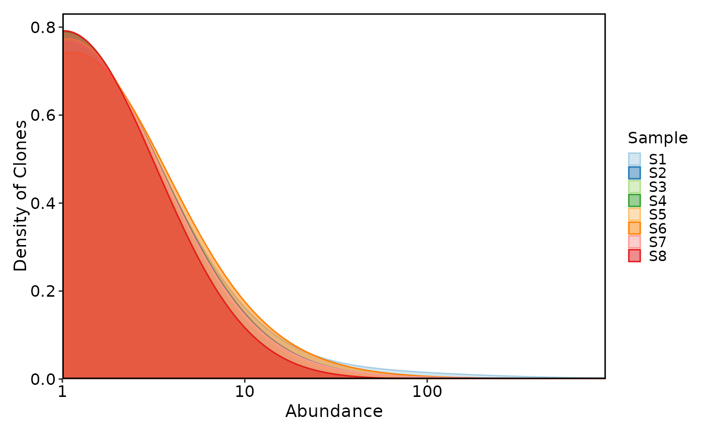
ClonalAbundancePlot(data, plot_type = "density")

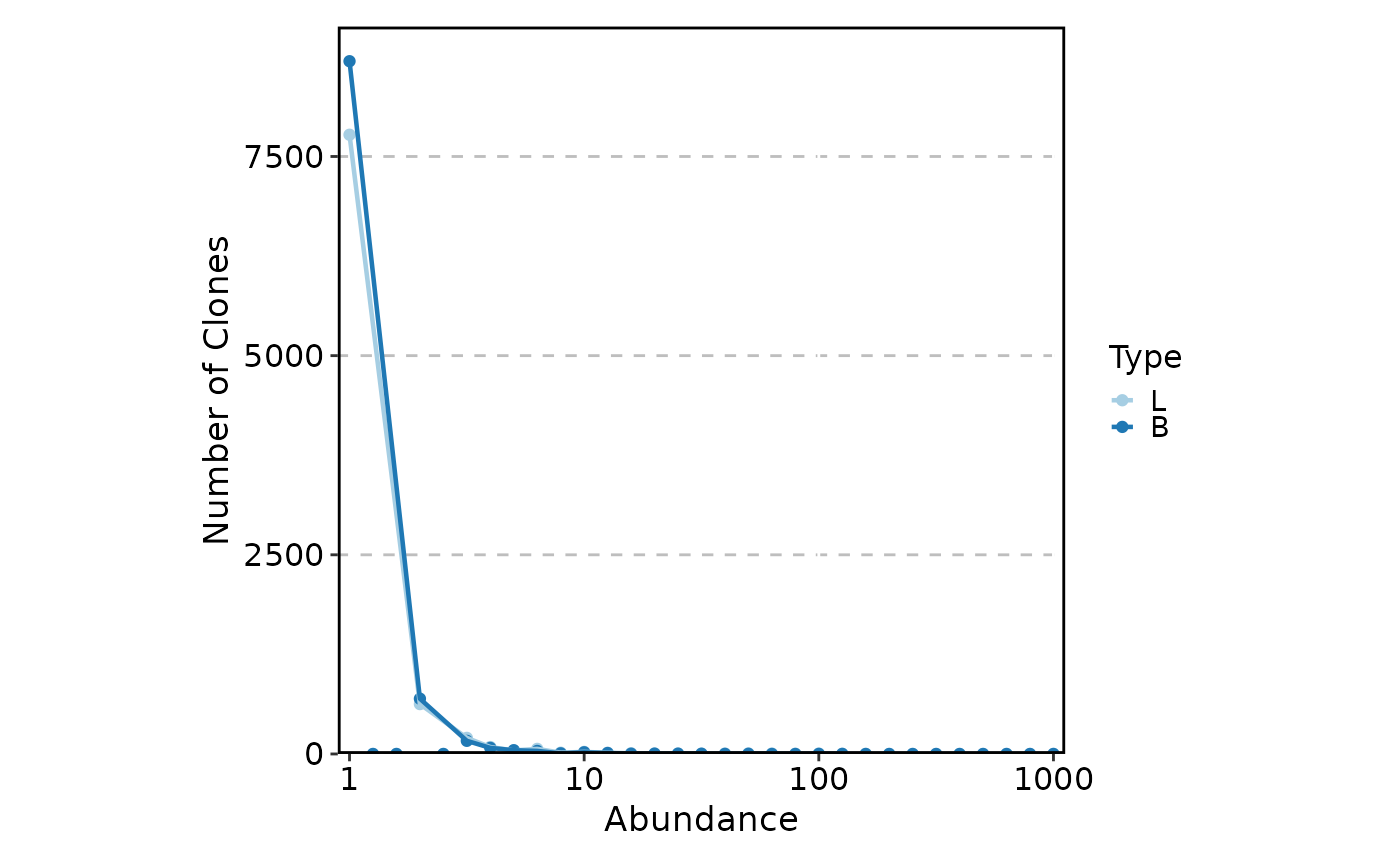
ClonalAbundancePlot(data, group_by = "Type")
#> Warning: Removed 9 rows containing missing values or values outside the scale range
#> (`geom_line()`).

# }