Density plot for visualising the distribution of a numeric variable. Uses
ggplot2::geom_density() to render smooth kernel density estimates, with
optional grouping, faceting, split-by splitting, and data-distribution rug
bars along the baseline.
This is the public entry point for density plots; the companion
Histogram() function provides binned-histogram rendering.
Both dispatch to the same internal engine (DensityHistoPlotAtomic)
with type = "density" or type = "histogram" respectively.
Histogram for visualising the distribution of a numeric variable via binned
counts. Uses ggplot2::geom_histogram(), with optional trend-line overlays,
zero-skip interpolation, grouping, faceting, and split-by splitting.
This is the histogram companion to DensityPlot(). Both dispatch to the
same internal engine (DensityHistoPlotAtomic) with type = "histogram"
or type = "density" respectively.
When use_trend = TRUE, the histogram bars are replaced entirely by a
point-and-line trend; when add_trend = TRUE, the trend is overlaid on top
of the bars. The trend_skip_zero option uses zoo::na.approx() to
interpolate across empty bins for a continuous trend curve — particularly
useful with transformed y-axes.
Usage
DensityPlot(
  data,
  x,
  group_by = NULL,
  group_by_sep = "_",
  group_name = NULL,
  xtrans = "identity",
  ytrans = "identity",
  split_by = NULL,
  split_by_sep = "_",
  flip = FALSE,
  position = "identity",
  palette = "Paired",
  palcolor = NULL,
  palreverse = FALSE,
  alpha = 0.5,
  theme = "theme_this",
  theme_args = list(),
  add_bars = FALSE,
  bar_height = 0.025,
  bar_alpha = 1,
  bar_width = 0.1,
  keep_na = FALSE,
  keep_empty = FALSE,
  title = NULL,
  subtitle = NULL,
  xlab = NULL,
  ylab = NULL,
  expand = c(bottom = 0, left = 0, right = 0),
  facet_by = NULL,
  facet_scales = "free_y",
  facet_ncol = NULL,
  facet_nrow = NULL,
  facet_byrow = TRUE,
  aspect.ratio = 1,
  legend.position = ifelse(is.null(group_by), "none", "right"),
  legend.direction = "vertical",
  seed = 8525,
  combine = TRUE,
  nrow = NULL,
  ncol = NULL,
  byrow = TRUE,
  axes = NULL,
  axis_titles = axes,
  guides = NULL,
  design = NULL,
  ...
)

Histogram(
  data,
  x,
  group_by = NULL,
  group_by_sep = "_",
  group_name = NULL,
  xtrans = "identity",
  ytrans = "identity",
  split_by = NULL,
  split_by_sep = "_",
  flip = FALSE,
  bins = NULL,
  binwidth = NULL,
  trend_skip_zero = FALSE,
  add_bars = FALSE,
  bar_height = 0.025,
  bar_alpha = 1,
  bar_width = 0.1,
  position = "identity",
  keep_na = FALSE,
  keep_empty = FALSE,
  use_trend = FALSE,
  add_trend = FALSE,
  trend_alpha = 1,
  trend_linewidth = 0.8,
  trend_pt_size = 1.5,
  palette = "Paired",
  palcolor = NULL,
  palreverse = FALSE,
  alpha = 0.5,
  theme = "theme_this",
  theme_args = list(),
  title = NULL,
  subtitle = NULL,
  xlab = NULL,
  ylab = NULL,
  expand = c(bottom = 0, left = 0, right = 0),
  facet_by = NULL,
  facet_scales = "free_y",
  facet_ncol = NULL,
  facet_nrow = NULL,
  facet_byrow = TRUE,
  aspect.ratio = 1,
  legend.position = ifelse(is.null(group_by), "none", "right"),
  legend.direction = "vertical",
  seed = 8525,
  combine = TRUE,
  nrow = NULL,
  ncol = NULL,
  byrow = TRUE,
  axes = NULL,
  axis_titles = axes,
  guides = NULL,
  design = NULL,
  ...
)
Arguments
- data
A data frame.
- x
A character string specifying the column name of the data frame to plot for the x-axis.
- group_by
Columns to group the data for plotting For those plotting functions that do not support multiple groups, They will be concatenated into one column, using
group_by_sepas the separator- group_by_sep
The separator for multiple group_by columns. See
group_by- group_name
A character string used as the legend title for the
group_byaesthetic. WhenNULL(default), the (possibly concatenated)group_bycolumn name is used.- xtrans
A character string specifying the transformation applied to the x-axis. Passed to
ggplot2::scale_x_continuous(transform = ...). Supported values include"identity"(default),"log10","log2","sqrt","reverse", etc.- ytrans
A character string specifying the transformation applied to the y-axis. Passed to
ggplot2::scale_y_continuous(transform = ...). Used bytrend_skip_zeroto correctly interpolate across zero bins on a transformed scale. Default:"identity".- split_by
The column(s) to split data by and plot separately.
- split_by_sep
The separator for multiple split_by columns. See
split_by- flip
A logical value. If
TRUE, the x and y axes are swapped viacoord_flip(). Dimension calculation accounts for the flip.- position
A character string specifying the position adjustment for the bars or density curves. Default:
"identity", which shows the actual count / density per group (unlikeggplot2's default"stack"). Other options:"stack","dodge","fill".- palette
A character string specifying the palette to use. A named list or vector can be used to specify the palettes for different
split_byvalues.- palcolor
A character string specifying the color to use in the palette. A named list can be used to specify the colors for different
split_byvalues. If some values are missing, the values from the palette will be used (palcolor will be NULL for those values).- palreverse
A logical value indicating whether to reverse the palette. Default is FALSE.
- alpha
A numeric value specifying the transparency of the plot.
- theme
A character string or a theme class (i.e. ggplot2::theme_classic) specifying the theme to use. Default is "theme_this".
- theme_args
A list of arguments to pass to the theme function.
- add_bars
A logical value. If
TRUE, a data-distribution rug is drawn along the y = 0 axis usinggeom_linerange(). Each group's bars are vertically offset to avoid overlap.- bar_height
A numeric value specifying the height (in data units, relative to the maximum y) of the rug bars added by
add_bars. The actual pixel height scales withmax_y. Default:0.025.- bar_alpha
A numeric value in
[0, 1]for the transparency of the rug bars. Default:1.- bar_width
A numeric value passed as the
linewidthaesthetic ofgeom_linerange(). Controls the thickness of each rug tick. Default:0.1.- keep_na
A logical value or a character to replace the NA values in the data. It can also take a named list to specify different behavior for different columns. If TRUE or NA, NA values will be replaced with NA. If FALSE, NA values will be removed from the data before plotting. If a character string is provided, NA values will be replaced with the provided string. If a named vector/list is provided, the names should be the column names to apply the behavior to, and the values should be one of TRUE, FALSE, or a character string. Without a named vector/list, the behavior applies to categorical/character columns used on the plot, for example, the
x,group_by,fill_by, etc.- keep_empty
One of FALSE, TRUE and "level". It can also take a named list to specify different behavior for different columns. Without a named list, the behavior applies to the categorical/character columns used on the plot, for example, the
x,group_by,fill_by, etc.FALSE(default): Drop empty factor levels from the data before plotting.TRUE: Keep empty factor levels and show them as a separate category in the plot."level": Keep empty factor levels, but do not show them in the plot. But they will be assigned colors from the palette to maintain consistency across multiple plots. Alias:levels
- title
A character string specifying the title of the plot. A function can be used to generate the title based on the default title. This is useful when split_by is used and the title needs to be dynamic.
- subtitle
A character string specifying the subtitle of the plot.
- xlab
A character string specifying the x-axis label.
- ylab
A character string specifying the y-axis label.
- expand
The values to expand the x and y axes. It is like CSS padding. When a single value is provided, it is used for both axes on both sides. When two values are provided, the first value is used for the top/bottom side and the second value is used for the left/right side. When three values are provided, the first value is used for the top side, the second value is used for the left/right side, and the third value is used for the bottom side. When four values are provided, the values are used for the top, right, bottom, and left sides, respectively. You can also use a named vector to specify the values for each side. When the axis is discrete, the values will be applied as 'add' to the 'expansion' function. When the axis is continuous, the values will be applied as 'mult' to the 'expansion' function. See also https://ggplot2.tidyverse.org/reference/expansion.html
- facet_by
A character string specifying the column name of the data frame to facet the plot. Otherwise, the data will be split by
split_byand generate multiple plots and combine them into one usingpatchwork::wrap_plots- facet_scales
Whether to scale the axes of facets. Default is "fixed" Other options are "free", "free_x", "free_y". See
ggplot2::facet_wrap- facet_ncol
A numeric value specifying the number of columns in the facet. When facet_by is a single column and facet_wrap is used.
- facet_nrow
A numeric value specifying the number of rows in the facet. When facet_by is a single column and facet_wrap is used.
- facet_byrow
A logical value indicating whether to fill the plots by row. Default is TRUE.
- aspect.ratio
A numeric value specifying the aspect ratio of the plot.
- legend.position
A character string specifying the position of the legend. if
waiver(), for single groups, the legend will be "none", otherwise "right".- legend.direction
A character string specifying the direction of the legend.
- seed
The random seed to use. Default is 8525.
- combine
Whether to combine the plots into one when facet is FALSE. Default is TRUE.
- nrow
A numeric value specifying the number of rows in the facet.
- ncol
A numeric value specifying the number of columns in the facet.
- byrow
A logical value indicating whether to fill the plots by row.
- axes
A string specifying how axes should be treated. Passed to
patchwork::wrap_plots(). Only relevant whensplit_byis used andcombineis TRUE. Options are:'keep' will retain all axes in individual plots.
'collect' will remove duplicated axes when placed in the same run of rows or columns of the layout.
'collect_x' and 'collect_y' will remove duplicated x-axes in the columns or duplicated y-axes in the rows respectively.
- axis_titles
A string specifying how axis titltes should be treated. Passed to
patchwork::wrap_plots(). Only relevant whensplit_byis used andcombineis TRUE. Options are:'keep' will retain all axis titles in individual plots.
'collect' will remove duplicated titles in one direction and merge titles in the opposite direction.
'collect_x' and 'collect_y' control this for x-axis titles and y-axis titles respectively.
- guides
A string specifying how guides should be treated in the layout. Passed to
patchwork::wrap_plots(). Only relevant whensplit_byis used andcombineis TRUE. Options are:'collect' will collect guides below to the given nesting level, removing duplicates.
'keep' will stop collection at this level and let guides be placed alongside their plot.
'auto' will allow guides to be collected if a upper level tries, but place them alongside the plot if not.
- design
Specification of the location of areas in the layout, passed to
patchwork::wrap_plots(). Only relevant whensplit_byis used andcombineis TRUE. When specified,nrow,ncol, andbyroware ignored. Seepatchwork::wrap_plots()for more details.- ...
Additional arguments.
- bins
A numeric value specifying the number of bins for the histogram. Ignored when
type = "density". Defaults to30when neitherbinsnorbinwidthis provided.- binwidth
A numeric value specifying the width of individual bins for the histogram. Ignored when
type = "density". Takes precedence overbinswhen both are set.- trend_skip_zero
A logical value. If
TRUE, bins with zero count are set toNAbefore the trend line is computed, andzoo::na.approx()is used to interpolate across the gaps — producing a continuous curve even when some bins are empty. Requiresytransto be correctly specified. Only applies whentype = "histogram"anduse_trendoradd_trendis active.- use_trend
A logical value. If
TRUE, the histogram bars are replaced entirely by a trend line (points + connecting line). Only applies whentype = "histogram".- add_trend
A logical value. If
TRUE, a trend line is overlaid on top of the histogram bars. Only applies whentype = "histogram".- trend_alpha
A numeric value in
[0, 1]controlling the transparency of the trend points and line. Default:1.- trend_linewidth
A numeric value for the thickness of the trend line. Default:
0.8.- trend_pt_size
A numeric value for the size of the trend points. Default:
1.5.
Value
A ggplot object (single plot), a patchwork / wrap_plots object
(when split_by is provided and combine = TRUE), or a list of ggplot
objects (when split_by is provided and combine = FALSE).
A ggplot object (single plot), a patchwork / wrap_plots object
(when split_by is provided and combine = TRUE), or a list of ggplot
objects (when split_by is provided and combine = FALSE).
split_by Workflow
When split_by is specified, DensityPlot() executes the following pipeline:
Argument validation —
validate_common_args()checks the seed and facet-by consistency.NA / empty normalisation —
check_keep_na()/check_keep_empty()convertkeep_na/keep_emptyto per-column lists.Theme resolution —
process_theme()resolves the theme string to a theme function.Split column resolution —
check_columns()validatessplit_by(force_factor, concat_multi).Pre-filtering —
process_keep_na_empty()removes NA / empty levels from the split column, thendatais split bysplit_bylevels (order preserved).Per-split parameter resolution —
check_palette(),check_palcolor(),check_legend()resolve palette, palcolor, legend.position, and legend.direction for each split.Per-split dispatch — each split is passed to
DensityHistoPlotAtomic(type = "density", ...)with its resolved parameters. Title defaults to the split level name unlesstitleis a function.Combination —
combine_plots()assembles the list of plots viapatchwork::wrap_plots(), applyingnrow,ncol,byrow,axes,axis_titles,guides, anddesign.
When split_by is specified, Histogram() executes the following pipeline:
Argument validation —
validate_common_args()checks the seed and facet-by consistency.NA / empty normalisation —
check_keep_na()/check_keep_empty()convertkeep_na/keep_emptyto per-column lists.Theme resolution —
process_theme()resolves the theme string to a theme function.Split column resolution —
check_columns()validatessplit_by(force_factor, concat_multi).Pre-filtering —
process_keep_na_empty()removes NA / empty levels from the split column, thendatais split bysplit_bylevels (order preserved).Per-split parameter resolution —
check_palette(),check_palcolor(),check_legend()resolve palette, palcolor, legend.position, and legend.direction for each split.Per-split dispatch — each split is passed to
DensityHistoPlotAtomic(type = "histogram", ...)with its resolved parameters (includingbins,binwidth,use_trend,add_trend,trend_skip_zero,trend_alpha,trend_linewidth,trend_pt_size). Title defaults to the split level name unlesstitleis a function.Combination —
combine_plots()assembles the list of plots viapatchwork::wrap_plots(), applyingnrow,ncol,byrow,axes,axis_titles,guides, anddesign.
Examples
# \donttest{
set.seed(8525)
data <- data.frame(
x = c(rnorm(500, -1), rnorm(500, 1)),
group = factor(rep(c("A", NA, "C", "D"), each = 250), levels = LETTERS[1:4]),
facet = sample(c("F1", "F2"), 1000, replace = TRUE)
)
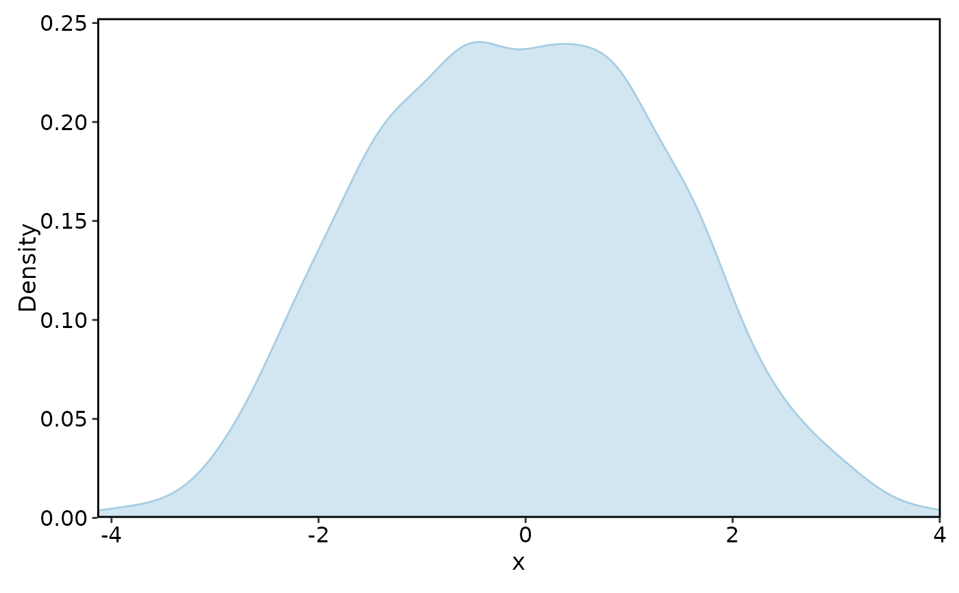
# basic density
DensityPlot(data, x = "x")
 DensityPlot(data, x = "x", group_by = "group")
 # NA / empty level handling
DensityPlot(data, x = "x", group_by = "group",
keep_na = TRUE, keep_empty = TRUE)
# NA / empty level handling
DensityPlot(data, x = "x", group_by = "group",
keep_na = TRUE, keep_empty = TRUE)
 DensityPlot(data, x = "x", group_by = "group",
keep_na = TRUE, keep_empty = 'level')
DensityPlot(data, x = "x", group_by = "group",
keep_na = TRUE, keep_empty = 'level')
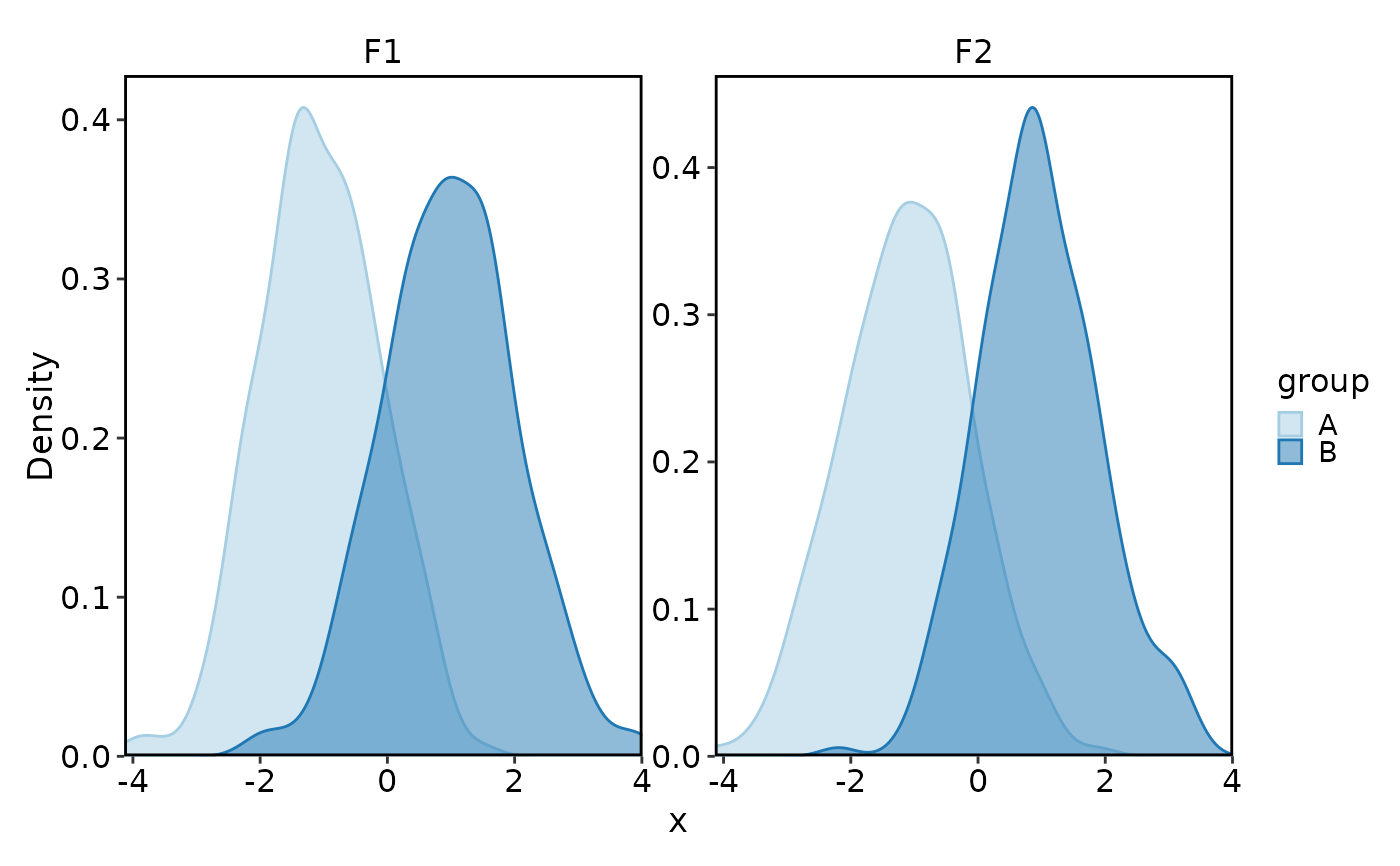
 # faceting and splitting
DensityPlot(data, x = "x", group_by = "group", facet_by = "facet")
# faceting and splitting
DensityPlot(data, x = "x", group_by = "group", facet_by = "facet")
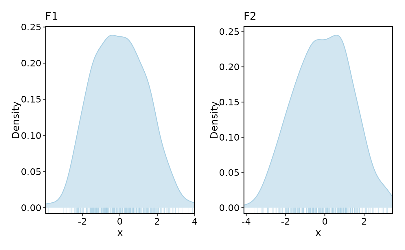
 DensityPlot(data, x = "x", split_by = "facet", add_bars = TRUE)
 DensityPlot(data, x = "x", split_by = "facet", add_bars = TRUE,
palette = c(F1 = "Set1", F2 = "Set2"))
DensityPlot(data, x = "x", split_by = "facet", add_bars = TRUE,
palette = c(F1 = "Set1", F2 = "Set2"))
 # }
set.seed(8525)
data <- data.frame(
x = sample(setdiff(1:100, c(30:36, 50:55, 70:77)), 1000, replace = TRUE),
group = factor(rep(c("A", "B", NA, "D"), each = 250), levels = LETTERS[1:4]),
facet = sample(c("F1", "F2"), 1000, replace = TRUE)
)
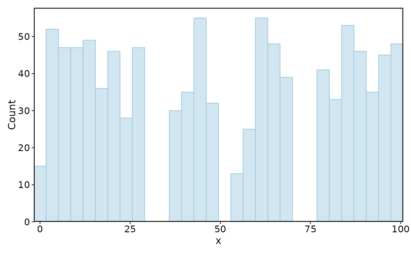
# basic histogram
Histogram(data, x = "x")
#> Using `bins = 30`. Pick better value with `binwidth`.
# }
set.seed(8525)
data <- data.frame(
x = sample(setdiff(1:100, c(30:36, 50:55, 70:77)), 1000, replace = TRUE),
group = factor(rep(c("A", "B", NA, "D"), each = 250), levels = LETTERS[1:4]),
facet = sample(c("F1", "F2"), 1000, replace = TRUE)
)
# basic histogram
Histogram(data, x = "x")
#> Using `bins = 30`. Pick better value with `binwidth`.
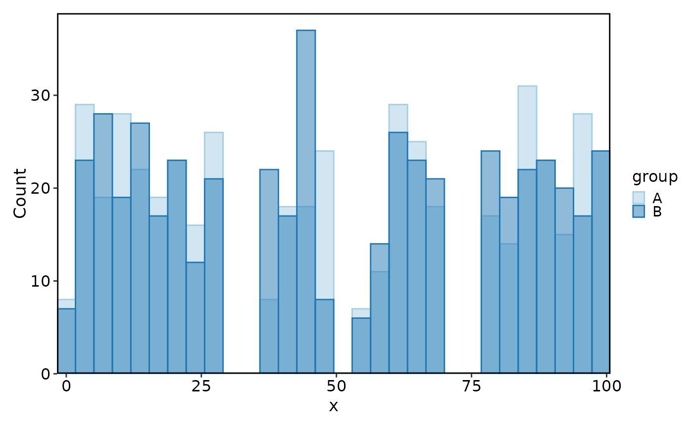
 Histogram(data, x = "x", group_by = "group")
#> Using `bins = 30`. Pick better value with `binwidth`.
Histogram(data, x = "x", group_by = "group")
#> Using `bins = 30`. Pick better value with `binwidth`.
 # NA / empty level handling
Histogram(data, x = "x", group_by = "group", keep_na = TRUE, keep_empty = 'level')
#> Using `bins = 30`. Pick better value with `binwidth`.
# NA / empty level handling
Histogram(data, x = "x", group_by = "group", keep_na = TRUE, keep_empty = 'level')
#> Using `bins = 30`. Pick better value with `binwidth`.
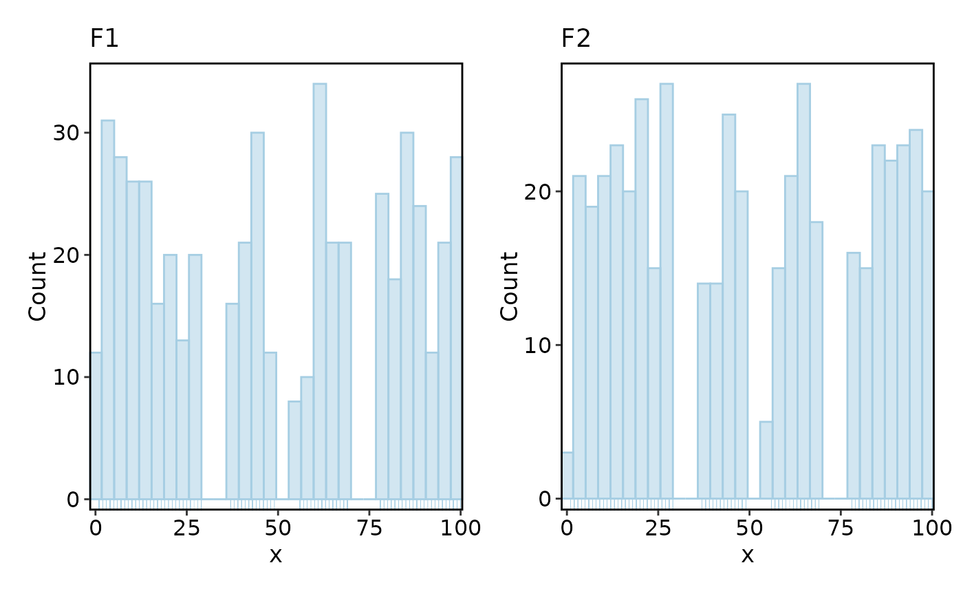
 # add_bars and trend overlays
Histogram(data, x = "x", split_by = "facet", add_bars = TRUE)
#> Using `bins = 30`. Pick better value with `binwidth`.
#> Using `bins = 30`. Pick better value with `binwidth`.
# add_bars and trend overlays
Histogram(data, x = "x", split_by = "facet", add_bars = TRUE)
#> Using `bins = 30`. Pick better value with `binwidth`.
#> Using `bins = 30`. Pick better value with `binwidth`.
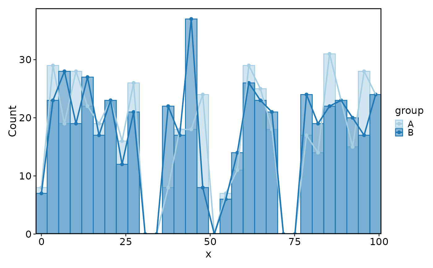
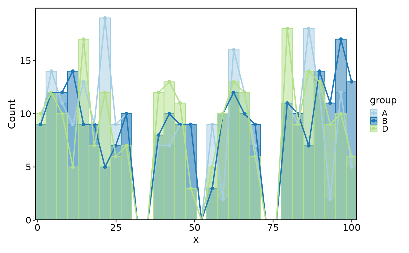
 Histogram(data, x = "x", group_by = "group", add_trend = TRUE)
#> Using `bins = 30`. Pick better value with `binwidth`.
Histogram(data, x = "x", group_by = "group", add_trend = TRUE)
#> Using `bins = 30`. Pick better value with `binwidth`.
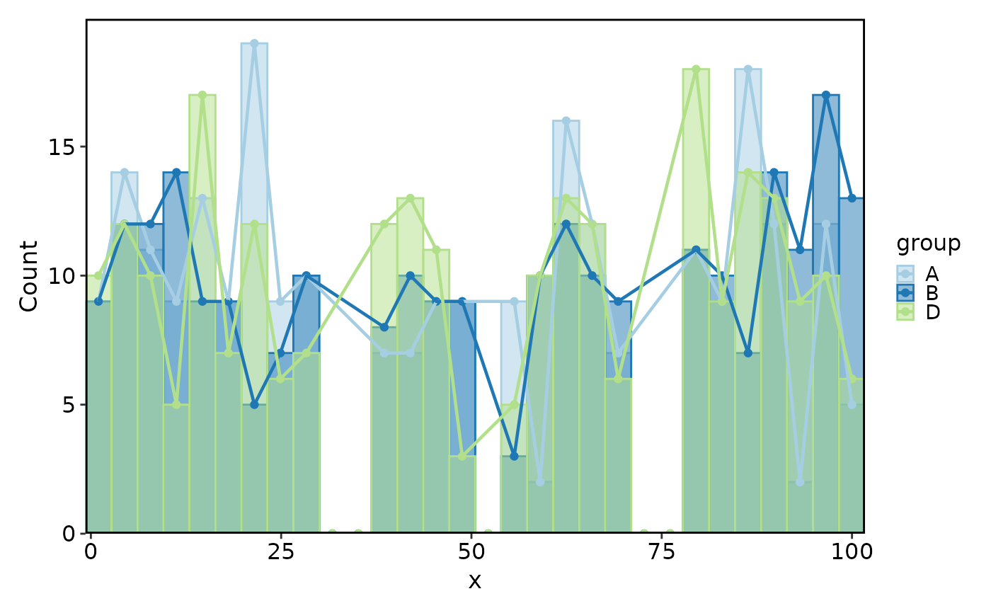
 Histogram(data, x = "x", group_by = "group", add_trend = TRUE, trend_skip_zero = TRUE)
#> Using `bins = 30`. Pick better value with `binwidth`.
Histogram(data, x = "x", group_by = "group", add_trend = TRUE, trend_skip_zero = TRUE)
#> Using `bins = 30`. Pick better value with `binwidth`.
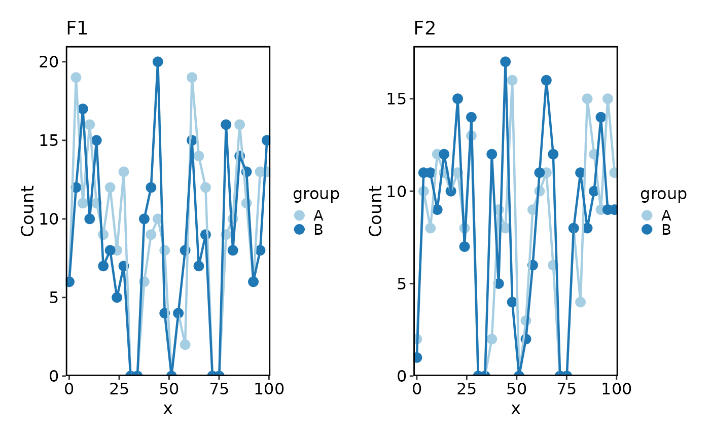
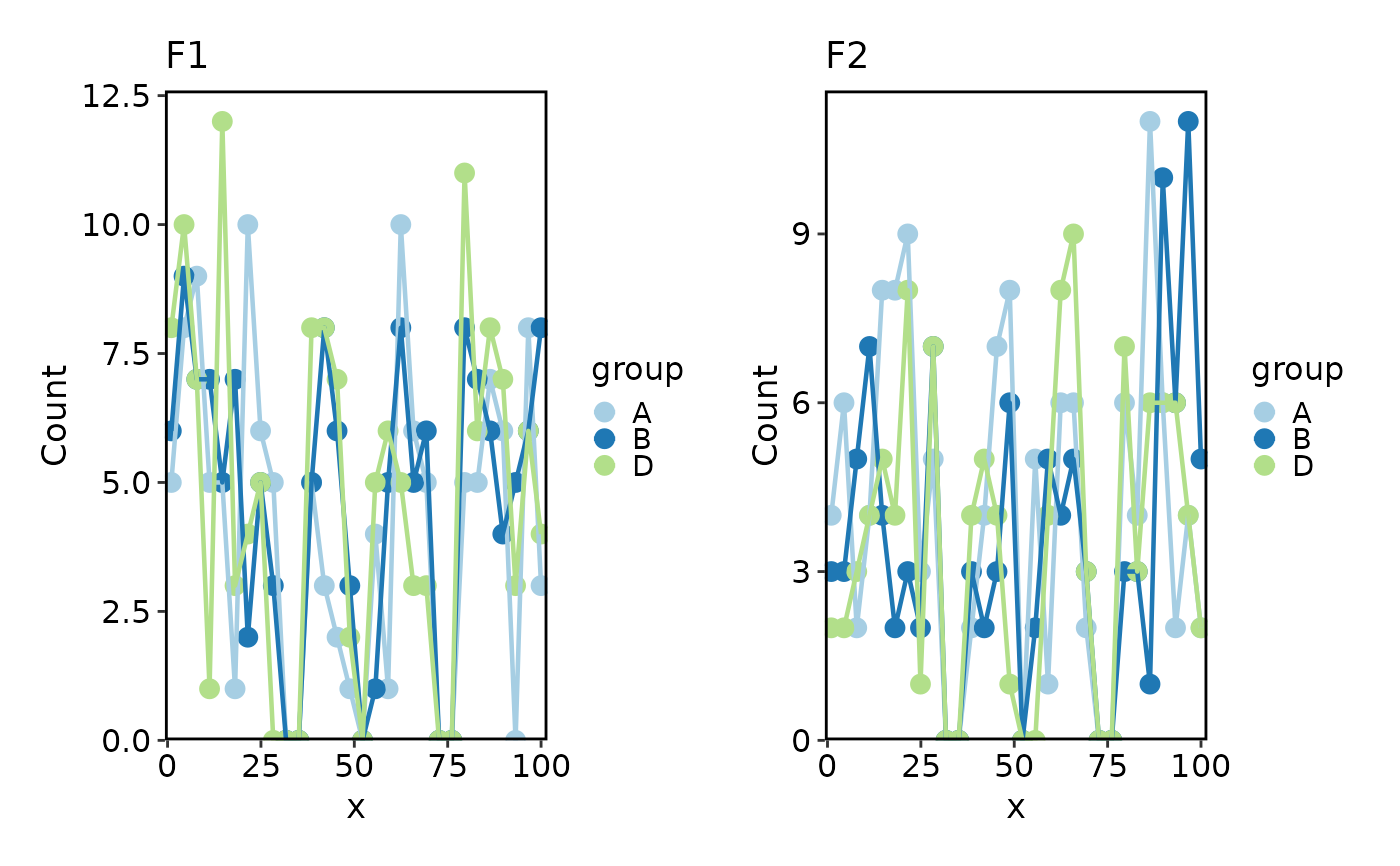
 # use_trend replaces bars entirely
Histogram(data, x = "x", group_by = "group", split_by = "facet",
use_trend = TRUE, trend_pt_size = 3)
#> Using `bins = 30`. Pick better value with `binwidth`.
#> Using `bins = 30`. Pick better value with `binwidth`.
# use_trend replaces bars entirely
Histogram(data, x = "x", group_by = "group", split_by = "facet",
use_trend = TRUE, trend_pt_size = 3)
#> Using `bins = 30`. Pick better value with `binwidth`.
#> Using `bins = 30`. Pick better value with `binwidth`.
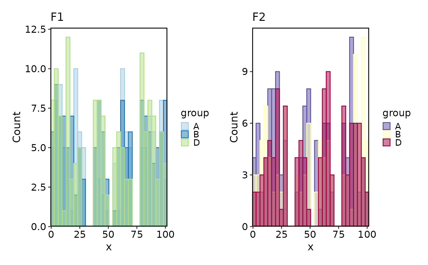
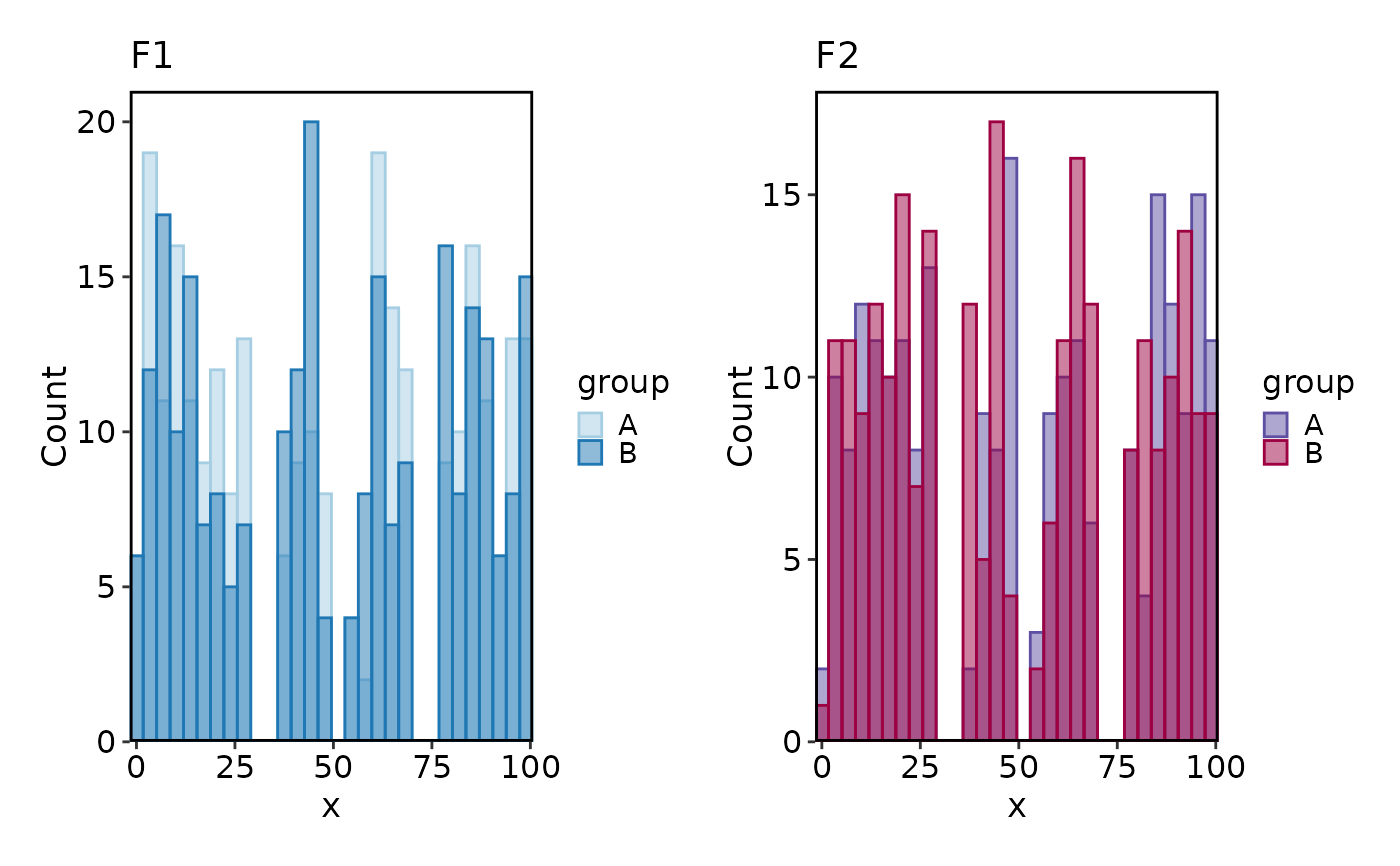
 # per-split palettes
Histogram(data, x = "x", group_by = "group", split_by = "facet",
palette = c(F1 = "Paired", F2 = "Spectral"))
#> Using `bins = 30`. Pick better value with `binwidth`.
#> Using `bins = 30`. Pick better value with `binwidth`.
# per-split palettes
Histogram(data, x = "x", group_by = "group", split_by = "facet",
palette = c(F1 = "Paired", F2 = "Spectral"))
#> Using `bins = 30`. Pick better value with `binwidth`.
#> Using `bins = 30`. Pick better value with `binwidth`.