QQ plot — QQPlot • plotthis

QQ plot is a graphical tool to compare two distributions by plotting their quantiles against each other.

Usage

QQPlot(
  data,
  val,
  val_trans = NULL,
  type = c("qq", "pp"),
  split_by = NULL,
  split_by_sep = "_",
  band = NULL,
  line = list(),
  point = list(),
  fill_name = "Bands",
  band_alpha = 0.5,
  theme = "theme_this",
  theme_args = list(),
  palette = "Spectral",
  palcolor = NULL,
  facet_by = NULL,
  facet_scales = "fixed",
  facet_ncol = NULL,
  facet_nrow = NULL,
  facet_byrow = TRUE,
  aspect.ratio = 1,
  legend.position = waiver(),
  legend.direction = "vertical",
  title = NULL,
  subtitle = NULL,
  xlim = NULL,
  ylim = NULL,
  xlab = ifelse(type == "qq", "Theoretical Quantiles", "Probability Points"),
  ylab = ifelse(type == "qq", "Sample Quantiles", "Cumulative Probability"),
  combine = TRUE,
  nrow = NULL,
  ncol = NULL,
  byrow = TRUE,
  seed = 8525,
  ...
)

Arguments

data: A data frame.
val: A character string of the column name for the values to plot. A numeric column is expected.
val_trans: A function to transform the values before plotting. Default is NULL, which means no transformation.
type: A character string to specify the type of plot. Default is "qq", which means QQ plot. Other options are "pp", which means PP plot.
split_by: The column(s) to split data by and plot separately.
split_by_sep: The separator for multiple split_by columns. See split_by
band: A list of arguments to pass to qqplotr::stat_qq_band() or qqplotr::stat_pp_band(), depending on the value of type. Default is NULL, which means no band. If an empty list or TRUE is provided, the default arguments will be used. Multiple bands can be added by providing a list of lists.
line: A list of arguments to pass to qqplotr::stat_qq_line() or qqplotr::stat_pp_line(), depending on the value of type. Default is list(), which means to add a line with default arguments. If NULL is provided, no line will be added.
point: A list of arguments to pass to qqplotr::stat_qq_point() or qqplotr::stat_pp_point(), depending on the value of type. Default is list(), which means to add points with default arguments. If NULL is provided, no points will be added (not recommended).
fill_name: A character string to name the legend of fill. Default is "Band Type".
band_alpha: A numeric value to set the alpha of all bands. Default is 0.5. It is a shortcut for setting alpha of all bands. You can override it by setting alpha in band argument. For example, band = list(list(alpha = 0.3), list(alpha = 0.7)).
theme: A character string or a theme class (i.e. ggplot2::theme_classic) specifying the theme to use. Default is "theme_this".
theme_args: A list of arguments to pass to the theme function.
palette: A character string specifying the palette to use. A named list or vector can be used to specify the palettes for different split_by values.
palcolor: A character string specifying the color to use in the palette. A named list can be used to specify the colors for different split_by values. If some values are missing, the values from the palette will be used (palcolor will be NULL for those values).
facet_by: A character string specifying the column name of the data frame to facet the plot. Otherwise, the data will be split by split_by and generate multiple plots and combine them into one using patchwork::wrap_plots
facet_scales: Whether to scale the axes of facets. Default is "fixed" Other options are "free", "free_x", "free_y". See ggplot2::facet_wrap
facet_ncol: A numeric value specifying the number of columns in the facet. When facet_by is a single column and facet_wrap is used.
facet_nrow: A numeric value specifying the number of rows in the facet. When facet_by is a single column and facet_wrap is used.
facet_byrow: A logical value indicating whether to fill the plots by row. Default is TRUE.
aspect.ratio: A numeric value specifying the aspect ratio of the plot.
legend.position: A character string specifying the position of the legend. if waiver(), for single groups, the legend will be "none", otherwise "right".
legend.direction: A character string specifying the direction of the legend.
title: A character string specifying the title of the plot. A function can be used to generate the title based on the default title. This is useful when split_by is used and the title needs to be dynamic.
subtitle: A character string specifying the subtitle of the plot.
xlim: A numeric vector of length 2 to set the x-axis limits.
ylim: A numeric vector of length 2 to set the y-axis limits.
xlab: A character string specifying the x-axis label.
ylab: A character string specifying the y-axis label.
combine: Whether to combine the plots into one when facet is FALSE. Default is TRUE.
nrow: A numeric value specifying the number of rows in the facet.
ncol: A numeric value specifying the number of columns in the facet.
byrow: A logical value indicating whether to fill the plots by row.
seed: The random seed to use. Default is 8525.
...: Additional arguments.

Value

A ggplot object or wrap_plots object or a list of ggplot objects

Examples

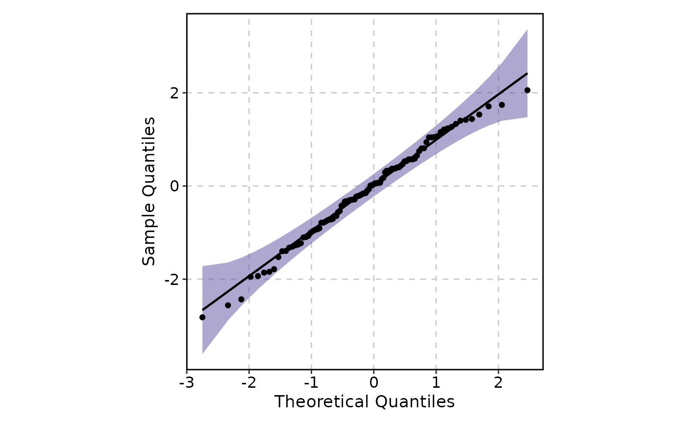
set.seed(8525)
data <- data.frame(norm = rnorm(100))

QQPlot(data, val = "norm", band = TRUE)

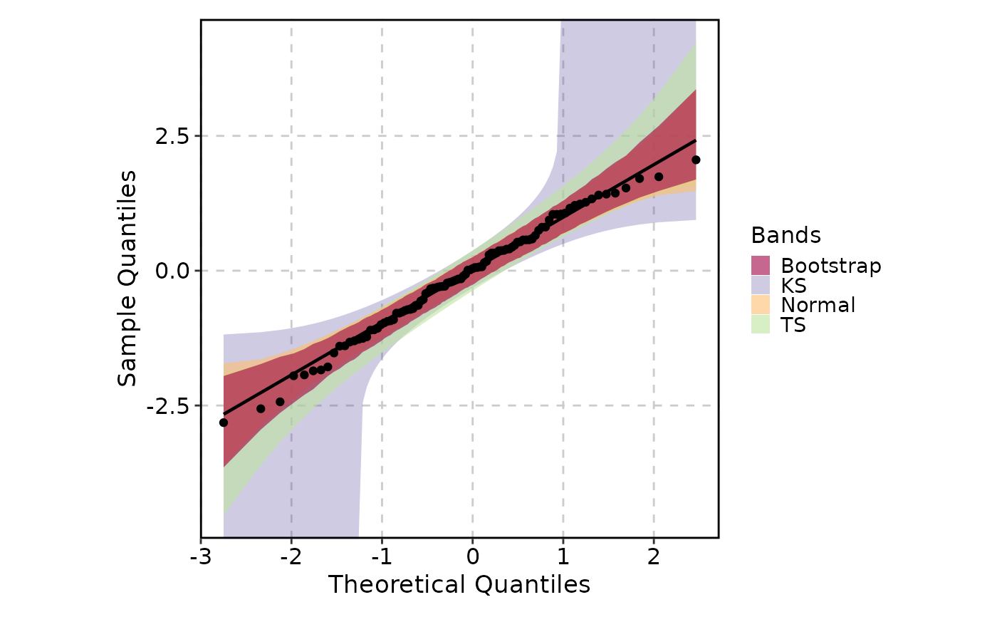
QQPlot(data, val = "norm", band = list(
    list(bandType = "ks", mapping = ggplot2::aes(fill = "KS"), alpha = 0.3),
    list(bandType = "ts", mapping = ggplot2::aes(fill = "TS")),
    list(bandType = "pointwise", mapping = ggplot2::aes(fill = "Normal")),
    list(bandType = "boot", mapping = ggplot2::aes(fill = "Bootstrap"))
), band_alpha = 0.6)


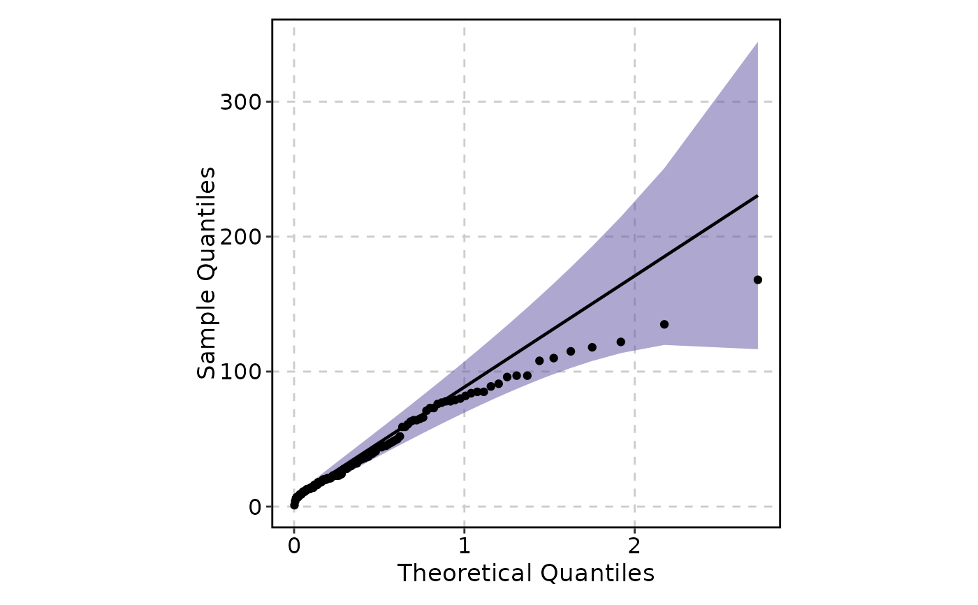
data(airquality, package = "datasets")
di <- "exp" # exponential distribution
dp <- list(rate = 2) # exponential rate parameter
QQPlot(airquality, val = "Ozone",
    band = list(distribution = di, dparams = dp),
    line = list(distribution = di, dparams = dp),
    point = list(distribution = di, dparams = dp)
)


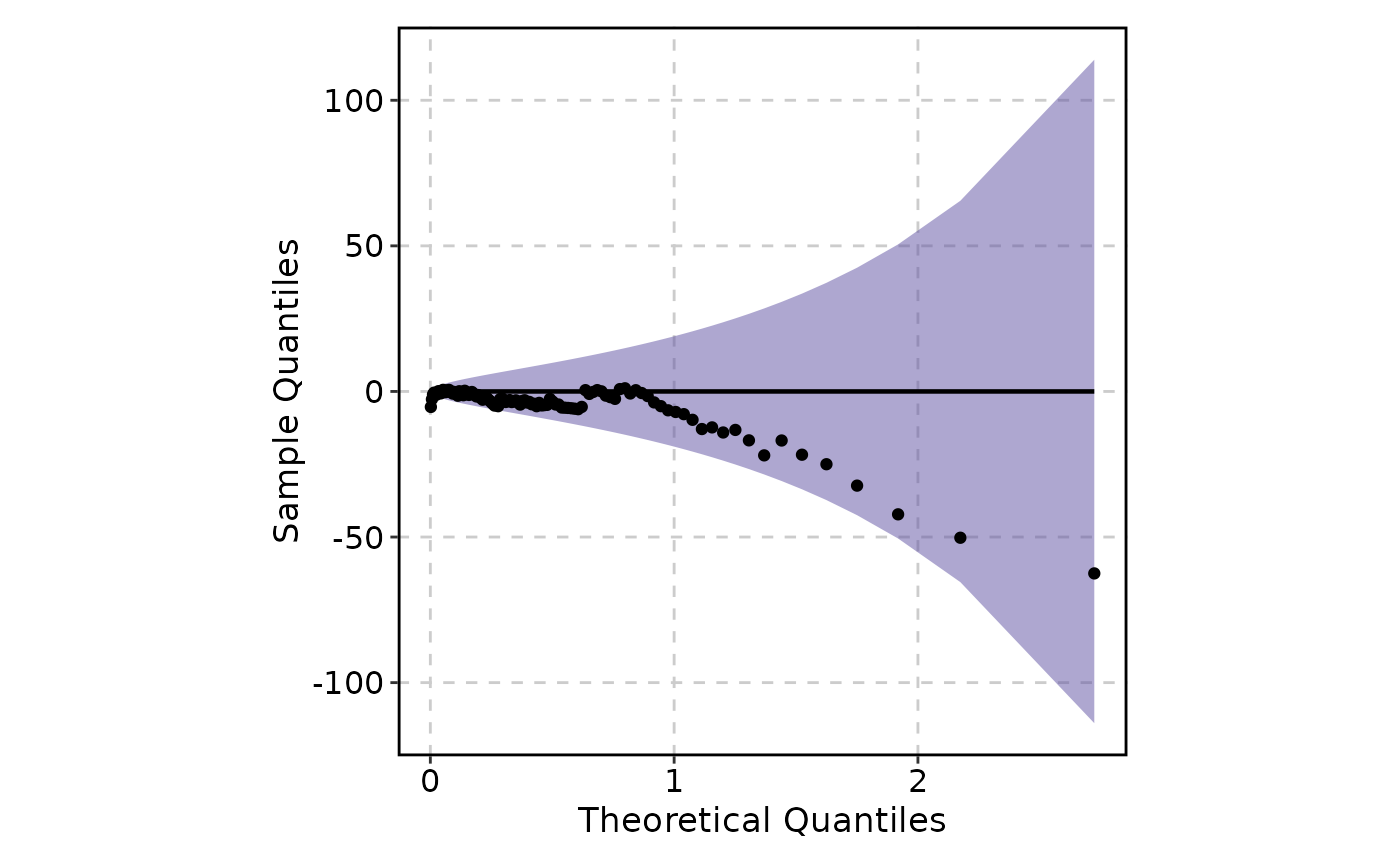
de <- TRUE # enabling the detrend option
QQPlot(airquality, val = "Ozone",
    band = list(distribution = di, dparams = dp, detrend = de),
    line = list(distribution = di, dparams = dp, detrend = de),
    point = list(distribution = di, dparams = dp, detrend = de)
)


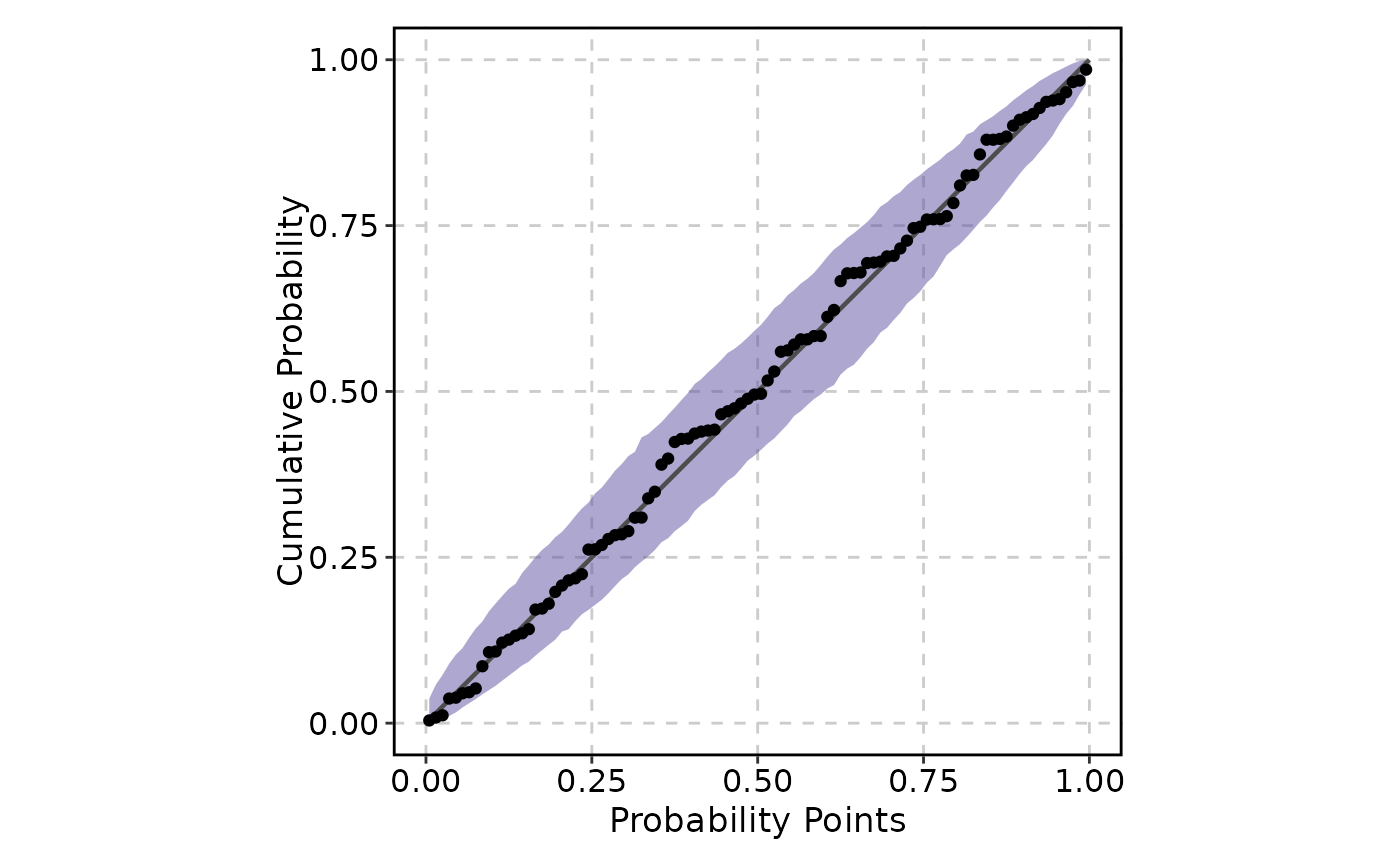
QQPlot(data, val = "norm", type = "pp", band = TRUE)


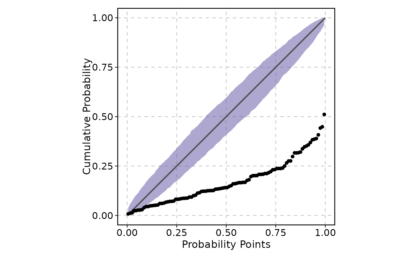
dp <- list(mean = 2, sd = 2) # shifted and rescaled Normal parameters
QQPlot(data, val = "norm", type = "pp",
    band = list(dparams = dp),
    point = list(dparams = dp))


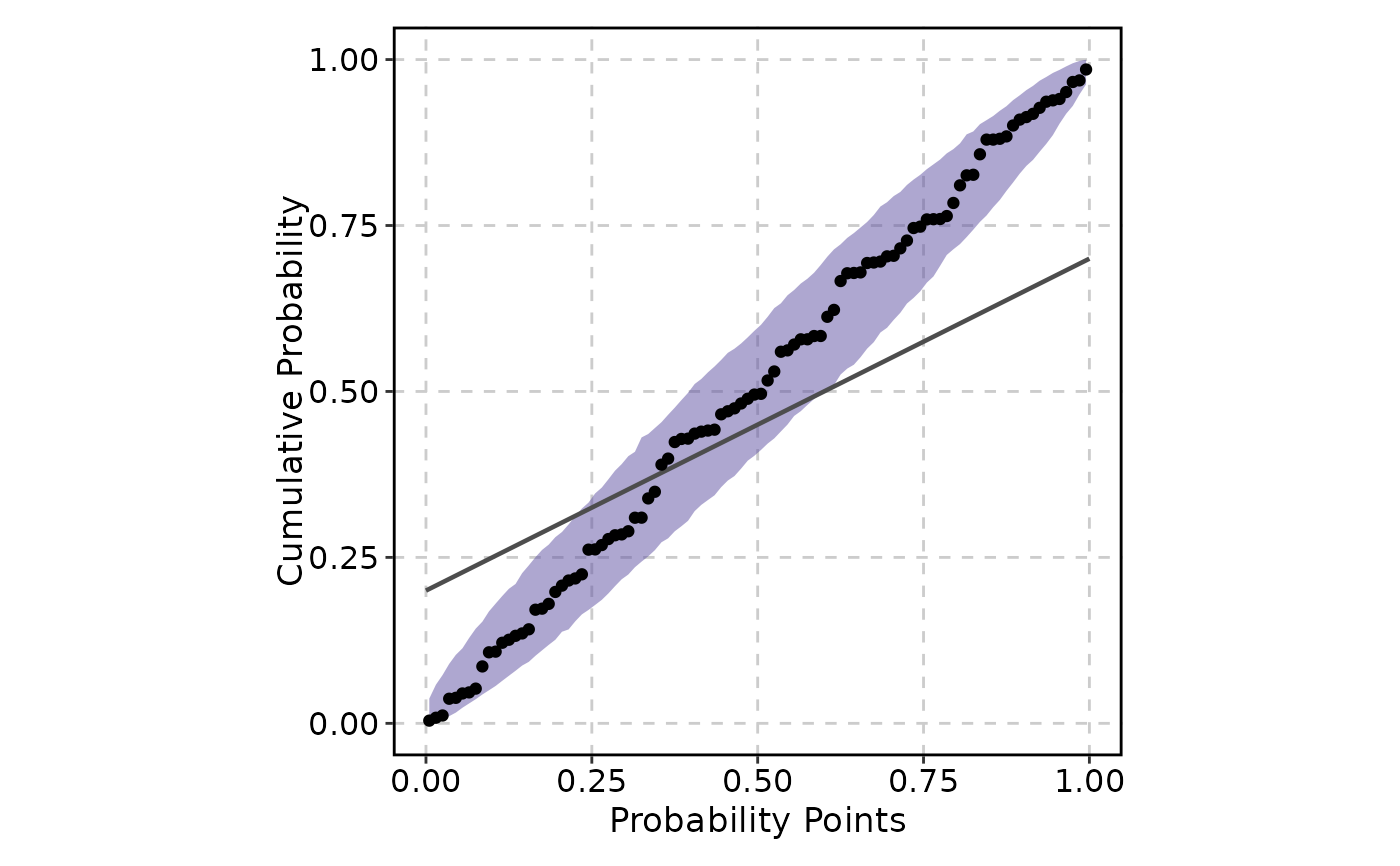
QQPlot(data, val = "norm", type = "pp", band = TRUE,
    line = list(ab = c(.2, .5)))


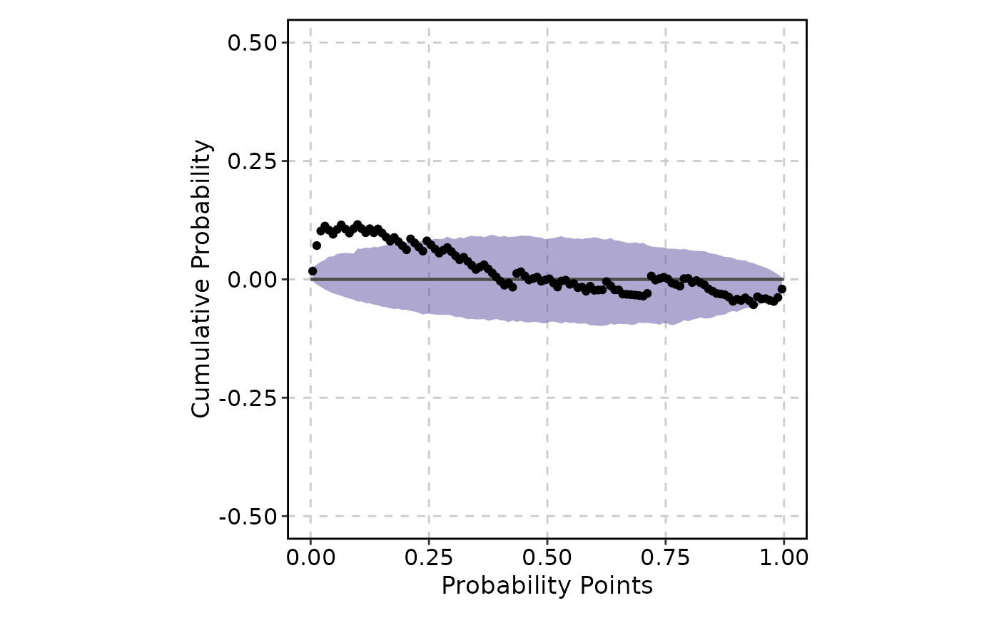
di <- "exp"
dp <- list(rate = .022) # value is based on some empirical tests
de <- TRUE
QQPlot(airquality, val = "Ozone", type = "pp",
   band = list(distribution = di, detrend = de, dparams = dp),
   line = list(detrend = de),
   point = list(distribution = di, detrend = de, dparams = dp),
   ylim = c(-.5, .5)
)