CloneResidency¶

Identification of clone residency

This process is used to investigate the residency of clones in groups, typically two samples (e.g. tumor and normal) from the same patient. But it can be used for any two groups of clones.

There are three types of output from this process

• Count tables of the clones in the two groups

  CDR3_aa	Tumor	Normal
  CASSYGLSWGSYEQYF	306	55
  CASSVTGAETQYF	295	37
  CASSVPSAHYNEQFF	197	9
  ...	...	...

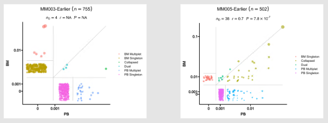
• Residency plots showing the residency of clones in the two groups

  

  The points in the plot are jittered to avoid overplotting. The x-axis is the residency in the first group and the y-axis is the residency in the second group. The size of the points are relative to the normalized size of the clones. You may identify different types of clones in the plot based on their residency in the two groups:
  

  • Collapsed (The clones that are collapsed in the second group)
  • Dual (The clones that are present in both groups with equal size)
  • Expanded (The clones that are expanded in the second group)
  • First Group Multiplet (The clones only in the First Group with size > 1)
  • Second Group Multiplet (The clones only in the Second Group with size > 1)
  • First Group Singlet (The clones only in the First Group with size = 1)
  • Second Group Singlet (The clones only in the Second Group with size = 1)

  This idea is borrowed from this paper:
  

  Wu, Thomas D., et al. "Peripheral T cell expansion predicts tumour infiltration and clinical response." Nature 579.7798 (2020): 274-278.

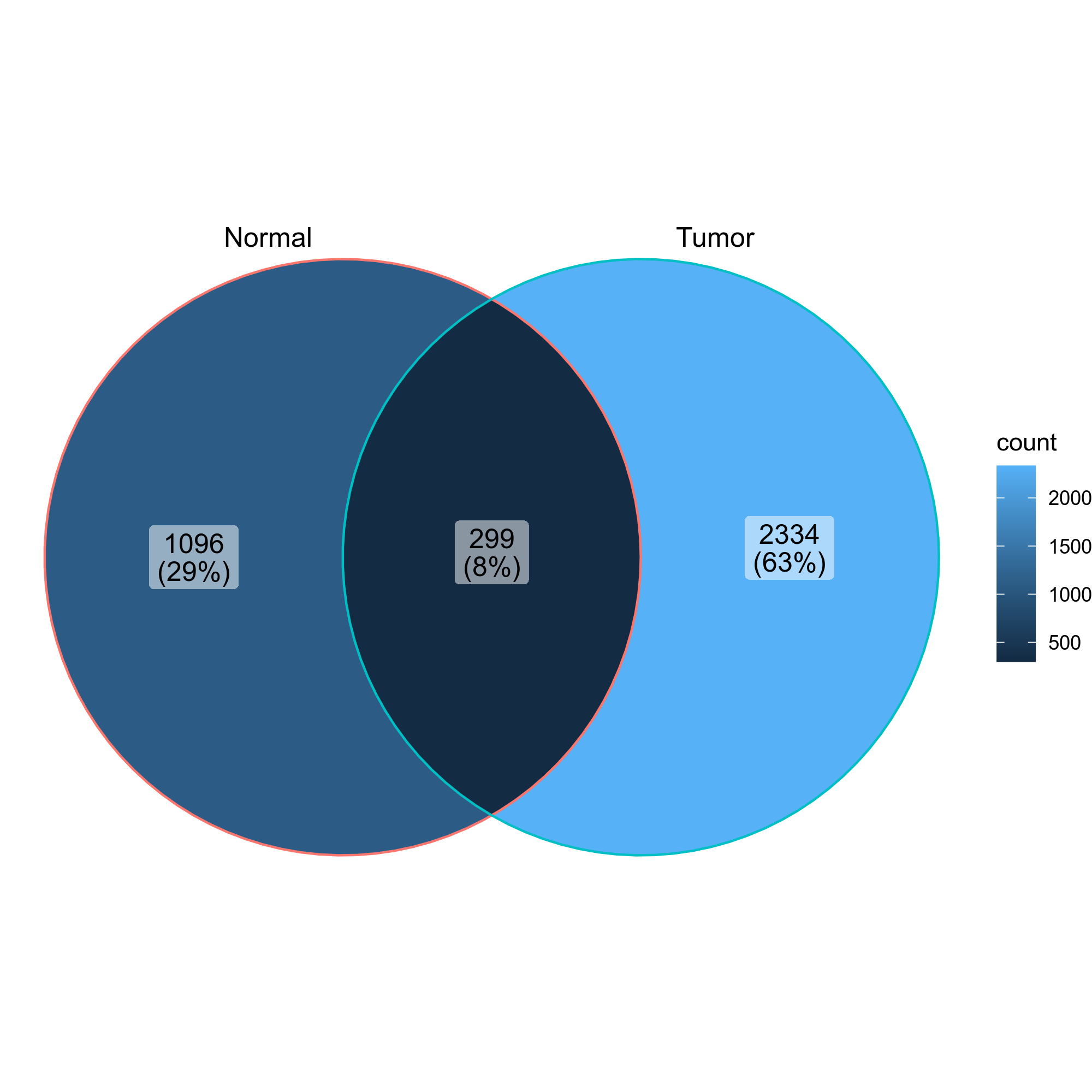
• Venn diagrams showing the overlap of the clones in the two groups

  

Environment Variables¶

• subject (list): Default: [].
  The key of subject in metadata. The clone residency will be examined for this subject/patient
• group: The key of group in metadata. This usually marks the samples that you want to compare. For example, Tumor vs Normal, post-treatment vs baseline It doesn't have to be 2 groups always. If there are more than 3 groups, instead of venn diagram, upset plots will be used.
  
• order (list): Default: [].
  The order of the values in group. In scatter/residency plots, X in X,Y will be used as x-axis and Y will be used as y-axis.
  You can also have multiple orders. For example: ["X,Y", "X,Z"].
  If you only have two groups, you can set order = ["X", "Y"], which will be the same as order = ["X,Y"].
  
• section: How the subjects aligned in the report. Multiple subjects with the same value will be grouped together.
  Useful for cohort with large number of samples.
  
• mutaters (type=json): Default: {}.
  The mutaters passed to dplyr::mutate() on the cell-level data converted from in.immdata. If in.metafile is provided, the mutaters will be applied to the joined data.
  The keys will be the names of the new columns, and the values will be the expressions. The new names can be used in subject, group, order and section.
  
• subset: The filter passed to dplyr::filter() to filter the data for the cells before calculating the clone residency. For example, Clones > 1 to filter out singletons.
  
• prefix: Default: {Sample}_.
  The prefix of the cell barcodes in the Seurat object.
  
• upset_ymax: The maximum value of the y-axis in the upset bar plots.
  
• upset_trans: The transformation to apply to the y axis of upset bar plots.
  For example, log10 or sqrt. If not specified, the y axis will be plotted as is. Note that the position of the bar plots will be dodged instead of stacked when the transformation is applied.
  See also https://github.com/tidyverse/ggplot2/issues/3671
• cases (type=json): Default: {}.
  If you have multiple cases, you can use this argument to specify them. The keys will be used as the names of the cases.
  The values will be passed to the corresponding arguments.
  If no cases are specified, the default case will be added, with the name DEFAULT and the values of envs.subject, envs.group, envs.order and envs.section. These values are also the defaults for the other cases.