"""Tools to analyze single-cell TCR sequencing data"""
from pipen.utils import mark
from ..core.defaults import SCRIPT_DIR
from ..core.proc import Proc
from ..core.config import config
@mark(deprecated="{proc.name} is deprecated, use ScRepLoading instead.")DOCS
class ImmunarchLoading(Proc):
"""Immuarch - Loading data
Load the raw data into [`immunarch`](https://immunarch.com) object,
using [`immunarch::repLoad()`](https://immunarch.com/reference/repLoad.html).
For the data path specified at `TCRData` in the input file, we will first find
`filtered_contig_annotations.csv` and `filtered_config_annotations.csv.gz` in the
path. If neighter of them exists, we will find `all_contig_annotations.csv` and
`all_contig_annotations.csv.gz` in the path and a warning will be raised
(You can find it at `./.pipen/<pipeline-name>/ImmunarchLoading/0/job.stderr`).
If none of the files exists, an error will be raised.
This process will also generate a text file with the information for each cell.
The file will be saved at
`./.pipen/<pipeline-name>/ImmunarchLoading/0/output/<prefix>.tcr.txt`.
The file can be used by the `SeuratMetadataMutater` process to integrate the
TCR-seq data into the `Seurat` object for further integrative analysis.
`envs.metacols` can be used to specify the columns to be exported to the text file.
Input:
metafile: The meta data of the samples
A tab-delimited file
Two columns are required:
* `Sample` to specify the sample names.
* `TCRData` to assign the path of the data to the samples,
and this column will be excluded as metadata.
Immunarch is able to fetch the sample names from the names of
the target files. However, 10x data yields result like
`filtered_contig_annotations.csv`, which doesn't have any name
information.
Output:
rdsfile: The RDS file with the data and metadata, which can be processed by
other `immunarch` functions.
metatxt: The meta data at cell level, which can be used to attach to the Seurat object
Envs:
prefix: The prefix to the barcodes. You can use placeholder like `{Sample}_`
to use the meta data from the `immunarch` object. The prefixed barcodes will
be saved in `out.metatxt`. The `immunarch` object keeps the original barcodes, but
the prefix is saved at `immdata$prefix`.
/// Note
This option is useful because the barcodes for the cells from scRNA-seq
data are usually prefixed with the sample name, for example,
`Sample1_AAACCTGAGAAGGCTA-1`. However, the barcodes for the cells from
scTCR-seq data are usually not prefixed with the sample name, for example,
`AAACCTGAGAAGGCTA-1`. So we need to add the prefix to the barcodes for
the scTCR-seq data, and it is easier for us to integrate the data from
different sources later.
///
tmpdir: The temporary directory to link all data files.
`Immunarch` scans a directory to find the data files. If the data files
are not in the same directory, we can link them to a temporary directory
and pass the temporary directory to `Immunarch`.
This option is useful when the data files are in different directories.
mode: Either "single" for single chain data or "paired" for
paired chain data. For `single`, only TRB chain will be kept
at `immdata$data`, information for other chains will be
saved at `immdata$tra` and `immdata$multi`.
extracols (list): The extra columns to be exported to the text file.
You can refer to the
[immunarch documentation](https://immunarch.com/articles/v2_data.html#immunarch-data-format)
to get a sense for the full list of the columns.
The columns may vary depending on the data source.
The columns from `immdata$meta` and some core columns, including
`Barcode`, `CDR3.aa`, `Clones`, `Proportion`, `V.name`, `J.name`, and
`D.name` will be exported by default. You can use this option to
specify the extra columns to be exported.
""" # noqa: E501
input = "metafile:file"
output = [
"rdsfile:file:{{in.metafile | stem}}.immunarch.RDS",
"metatxt:file:{{in.metafile | stem}}.tcr.txt",
]
lang = config.lang.rscript
envs = {
"tmpdir": config.path.tmpdir,
"prefix": "{Sample}_",
"mode": "paired",
"extracols": [],
}
script = "file://../scripts/tcr/ImmunarchLoading.R"
@mark(deprecated=True)DOCS
class ImmunarchFilter(Proc):
"""Immunarch - Filter data
See <https://immunarch.com/articles/web_only/repFilter_v3.html>
Input:
immdata: The data loaded by `immunarch::repLoad()`
filterfile: A config file in TOML.
A dict of configurations with keys as the names of the group and
values dicts with following keys.
See `envs.filters`
Output:
outfile: The filtered `immdata`
groupfile: Also a group file with rownames as cells and column names as
each of the keys in `in.filterfile` or `envs.filters`. The values
will be subkeys of the dicts in `in.filterfile` or `envs.filters`.
Envs:
filters: The filters to filter the data
You can have multiple cases (groups), the names will be the keys of
this dict, values are also dicts with keys the methods supported by
`immunarch::repFilter()`.
There is one more method `by.count` supported to filter the
count matrix. For `by.meta`, `by.repertoire`, `by.rep`,
`by.clonotype` or `by.col` the values will be passed to
`.query` of `repFilter()`.
You can also use the helper functions provided by `immunarch`,
including `morethan`, `lessthan`, `include`, `exclude` and
`interval`. If these functions are not used, `include(value)` will
be used by default.
For `by.count`, the value of `filter` will be passed to
`dplyr::filter()` to filter the count matrix.
You can also specify `ORDER` to define the filtration order, which
defaults to 0, higher `ORDER` gets later executed.
Each subkey/subgroup must be exclusive
For example:
>>> {
>>> "name": "BM_Post_Clones",
>>> "filters" {
>>> "Top_20": {
>>> "SAVE": True, # Save the filtered data to immdata
>>> "by.meta": {"Source": "BM", "Status": "Post"},
>>> "by.count": {
>>> "ORDER": 1, "filter": "TOTAL %%in%% TOTAL[1:20]"
>>> }
>>> },
>>> "Rest": {
>>> "by.meta": {"Source": "BM", "Status": "Post"},
>>> "by.count": {
>>> "ORDER": 1, "filter": "!TOTAL %%in%% TOTAL[1:20]"
>>> }
>>> }
>>> }
prefix: The prefix will be added to the cells in the output file
Placeholders like `{Sample}_` can be used to from the meta data
metacols: The extra columns to be exported to the group file.
"""
input = "immdata:file, filterfile:file"
output = """
outfile:file:{{in.immdata | stem}}.RDS,
groupfile:file:{% if in.filterfile -%}
{{- in.filterfile | toml_load | attr: "name" | append: ".txt" -}}
{%- else -%}
{{- envs.filters | attr: "name" | append: ".txt" -}}
{%- endif -%}
"""
envs = {
"prefix": "{Sample}_",
"filters": {},
"metacols": ["Clones", "Proportion", "CDR3.aa"],
}
lang = config.lang.rscript
script = "file://../scripts/tcr/ImmunarchFilter.R"
@mark(deprecated="{proc.name} is deprecated, use ClonalStats instead.")DOCS
class Immunarch(Proc):
"""Exploration of Single-cell and Bulk T-cell/Antibody Immune Repertoires
See <https://immunarch.com/articles/web_only/v3_basic_analysis.html>
After [`ImmunarchLoading`](!!#biopipennstcrimmunarchloading) loads the raw data into an [immunarch](https://immunarch.com) object,
this process wraps the functions from [`immunarch`](https://immunarch.com) to do the following:
- Basic statistics, provided by [`immunarch::repExplore`](https://immunarch.com/reference/repExplore.html), such as number of clones or distributions of lengths and counts.
- The clonality of repertoires, provided by [`immunarch::repClonality`](https://immunarch.com/reference/repClonality.html)
- The repertoire overlap, provided by [`immunarch::repOverlap`](https://immunarch.com/reference/repOverlap.html)
- The repertoire overlap, including different clustering procedures and PCA, provided by [`immunarch::repOverlapAnalysis`](https://immunarch.com/reference/repOverlapAnalysis.html)
- The distributions of V or J genes, provided by [`immunarch::geneUsage`](https://immunarch.com/reference/geneUsage.html)
- The diversity of repertoires, provided by [`immunarch::repDiversity`](https://immunarch.com/reference/repDiversity.html)
- The dynamics of repertoires across time points/samples, provided by [`immunarch::trackClonotypes`](https://immunarch.com/reference/trackClonotypes.html)
- The spectratype of clonotypes, provided by [`immunarch::spectratype`](https://immunarch.com/reference/spectratype.html)
- The distributions of kmers and sequence profiles, provided by [`immunarch::getKmers`](https://immunarch.com/reference/getKmers.html)
- The V-J junction circos plots, implemented within the script of this process.
Environment Variable Design:
With different sets of arguments, a single function of the above can perform different tasks.
For example, `repExplore` can be used to get the statistics of the size of the repertoire,
the statistics of the length of the CDR3 region, or the statistics of the number of
the clonotypes. Other than that, you can also have different ways to visualize the results,
by passing different arguments to the [`immunarch::vis`](https://immunarch.com/reference/vis.html) function.
For example, you can pass `.by` to `vis` to visualize the results of `repExplore` by different groups.
Before we explain each environment variable in details in the next section, we will give some examples here to show how the environment variables are organized in order for a single function to perform different tasks.
```toml
# Repertoire overlapping
[Immunarch.envs.overlaps]
# The method to calculate the overlap, passed to `repOverlap`
method = "public"
```
What if we want to calculate the overlap by different methods at the same time? We can use the following configuration:
```toml
[Immunarch.envs.overlaps.cases]
Public = { method = "public" }
Jaccard = { method = "jaccard" }
```
Then, the `repOverlap` function will be called twice, once with `method = "public"` and once with `method = "jaccard"`. We can also use different arguments to visualize the results. These arguments will be passed to the `vis` function:
```toml
[Immunarch.envs.overlaps.cases.Public]
method = "public"
vis_args = { "-plot": "heatmap2" }
[Immunarch.envs.overlaps.cases.Jaccard]
method = "jaccard"
vis_args = { "-plot": "heatmap2" }
```
`-plot` will be translated to `.plot` and then passed to `vis`.
If multiple cases share the same arguments, we can use the following configuration:
```toml
[Immunarch.envs.overlaps]
vis_args = { "-plot": "heatmap2" }
[Immunarch.envs.overlaps.cases]
Public = { method = "public" }
Jaccard = { method = "jaccard" }
```
For some results, there are futher analysis that can be performed. For example, for the repertoire overlap, we can perform clustering and PCA (see also <https://immunarch.com/articles/web_only/v4_overlap.html>):
```R
imm_ov1 <- repOverlap(immdata$data, .method = "public", .verbose = F)
repOverlapAnalysis(imm_ov1, "mds") %>% vis()
repOverlapAnalysis(imm_ov1, "tsne") %>% vis()
```
In such a case, we can use the following configuration:
```toml
[Immunarch.envs.overlaps]
method = "public"
[Immunarch.envs.overlaps.analyses.cases]
MDS = { "-method": "mds" }
TSNE = { "-method": "tsne" }
```
Then, the `repOverlapAnalysis` function will be called twice on the result generated by `repOverlap(immdata$data, .method = "public")`, once with `.method = "mds"` and once with `.method = "tsne"`. We can also use different arguments to visualize the results. These arguments will be passed to the `vis` function:
```toml
[Immunarch.envs.overlaps]
method = "public"
[Immunarch.envs.overlaps.analyses]
# See: <https://immunarch.com/reference/vis.immunr_hclust.html>
vis_args = { "-plot": "best" }
[Immunarch.envs.overlaps.analyses.cases]
MDS = { "-method": "mds" }
TSNE = { "-method": "tsne" }
```
Generally, you don't need to specify `cases` if you only have one case. A default case will be created for you. For multiple cases, the arguments at the same level as `cases` will be inherited by all cases.
Examples:
```toml
[Immunarch.envs.kmers]
k = 5
```
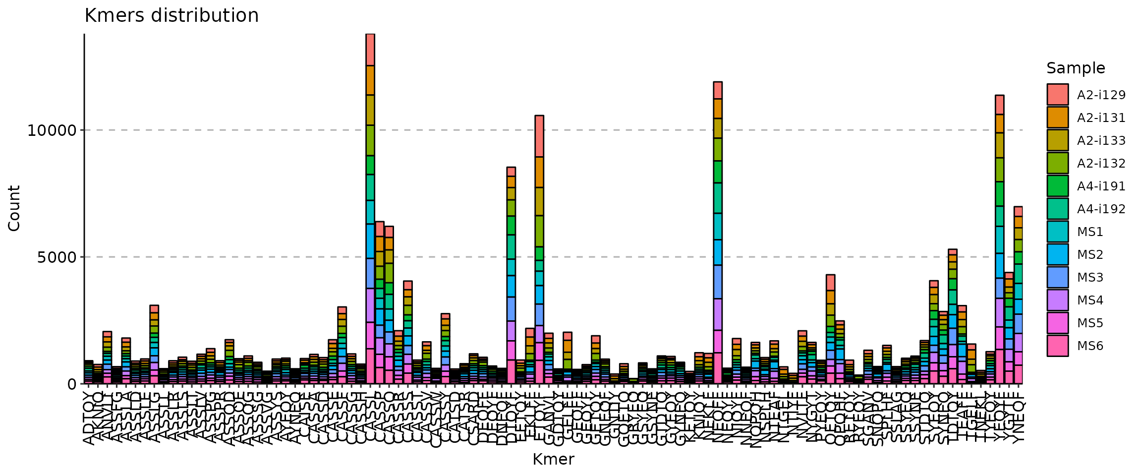
```toml
[Immunarch.envs.kmers]
# Shared by cases
k = 5
[Immunarch.envs.kmers.cases]
Head5 = { head = 5, -position = "stack" }
Head10 = { head = 10, -position = "fill" }
Head30 = { head = 30, -position = "dodge" }
```
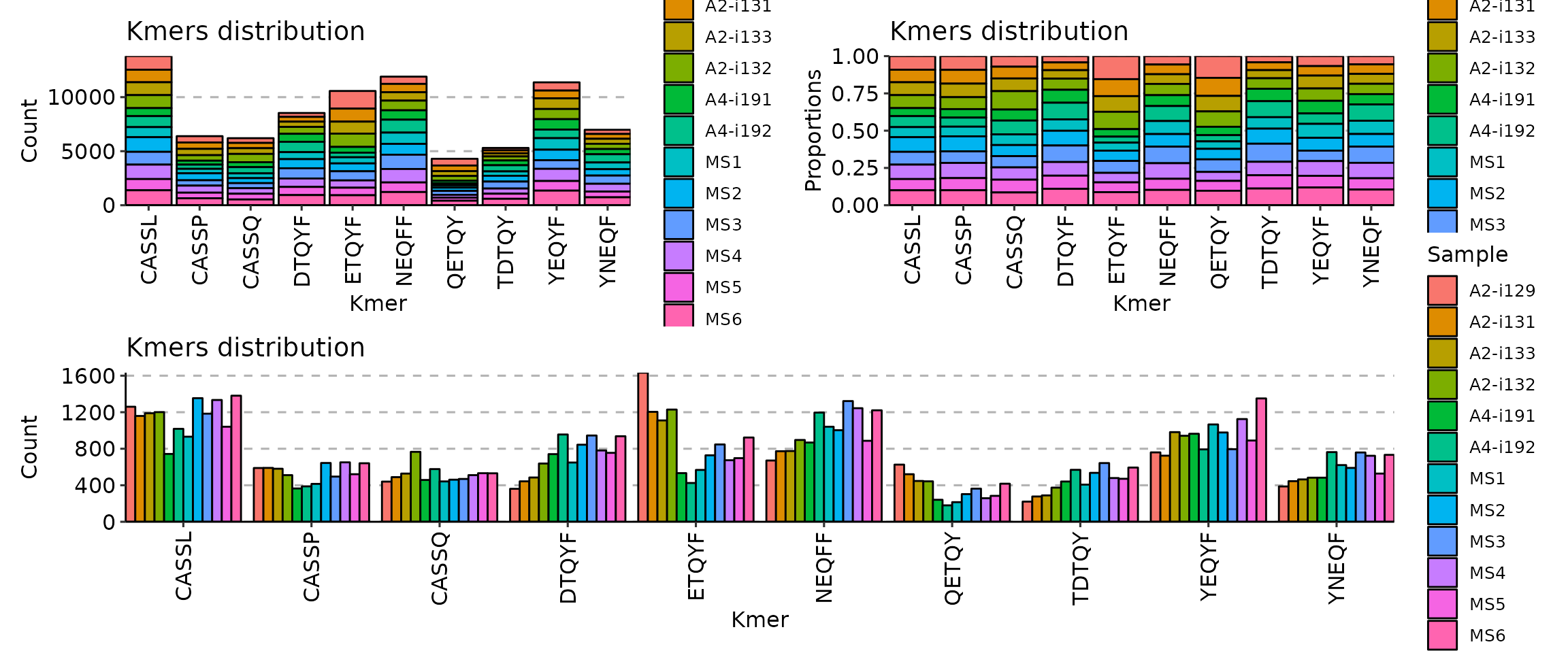
With motif profiling:
```toml
[Immunarch.envs.kmers]
k = 5
[Immnuarch.envs.kmers.profiles.cases]
TextPlot = { method = "self", vis_args = { "-plot": "text" } }
SeqPlot = { method = "self", vis_args = { "-plot": "seq" } }
```
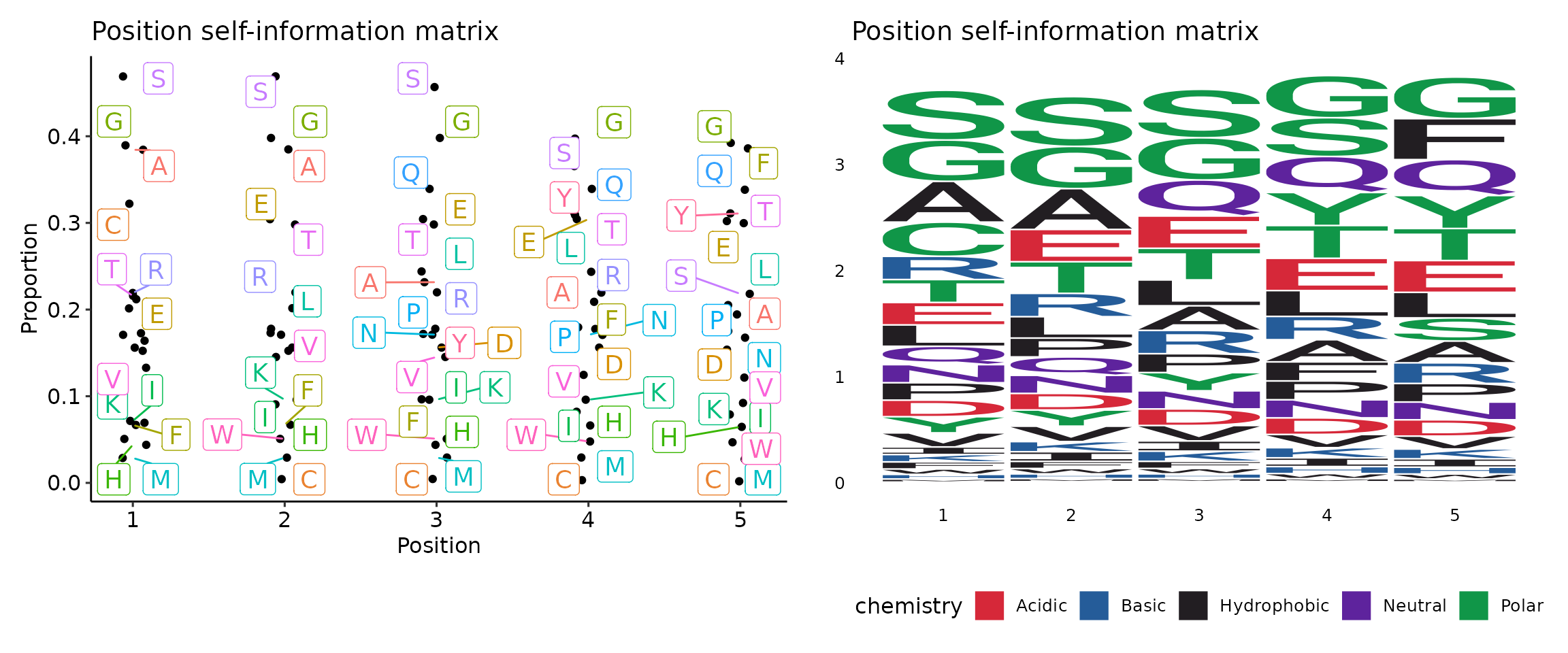
Input:
immdata: The data loaded by `immunarch::repLoad()`
metafile: A cell-level metafile, where the first column must be the cell barcodes
that match the cell barcodes in `immdata`. The other columns can be any
metadata that you want to use for the analysis. The loaded metadata will be
left-joined to the converted cell-level data from `immdata`.
This can also be a Seurat object RDS file. If so, the `sobj@meta.data` will
be used as the metadata.
Output:
outdir: The output directory
Envs:
mutaters (type=json;order=-9): The mutaters passed to `dplyr::mutate()` on expanded cell-level data
to add new columns.
The keys will be the names of the columns, and the values will be the expressions.
The new names can be used in `volumes`, `lens`, `counts`, `top_clones`, `rare_clones`, `hom_clones`, `gene_usages`, `divs`, etc.
prefix: The prefix to the barcodes. You can use placeholder like `{Sample}_`
The prefixed barcodes will be used to match the barcodes in `in.metafile`.
Not used if `in.metafile` is not specified.
If `None` (default), `immdata$prefix` will be used.
volumes (ns): Explore clonotype volume (sizes).
- by: Groupings when visualize clonotype volumes, passed to the `.by` argument of `vis(imm_vol, .by = <values>)`.
Multiple columns should be separated by `,`.
- devpars (ns): The parameters for the plotting device.
- width (type=int): The width of the plot.
- height (type=int): The height of the plot.
- res (type=int): The resolution of the plot.
- subset: Subset the data before calculating the clonotype volumes.
The whole data will be expanded to cell level, and then subsetted.
Clone sizes will be re-calculated based on the subsetted data.
- cases (type=json;order=9): If you have multiple cases, you can use this argument to specify them.
The keys will be the names of the cases.
The values will be passed to the corresponding arguments above.
If any of these arguments are not specified, the values in `envs.volumes` will be used.
If NO cases are specified, the default case will be added, with the name `DEFAULT` and the
values of `envs.volume.by`, `envs.volume.devpars`.
lens (ns): Explore clonotype CDR3 lengths.
- by: Groupings when visualize clonotype lengths, passed to the `.by` argument of `vis(imm_len, .by = <values>)`.
Multiple columns should be separated by `,`.
- devpars (ns): The parameters for the plotting device.
- width (type=int): The width of the plot.
- height (type=int): The height of the plot.
- res (type=int): The resolution of the plot.
- subset: Subset the data before calculating the clonotype volumes.
The whole data will be expanded to cell level, and then subsetted.
Clone sizes will be re-calculated based on the subsetted data.
- cases (type=json;order=9): If you have multiple cases, you can use this argument to specify them.
The keys will be the names of the cases.
The values will be passed to the corresponding arguments above.
If any of these arguments are not specified, the values in `envs.lens` will be used.
If NO cases are specified, the default case will be added, with the name `DEFAULT` and the
values of `envs.lens.by`, `envs.lens.devpars`.
counts (ns): Explore clonotype counts.
- by: Groupings when visualize clonotype counts, passed to the `.by` argument of `vis(imm_count, .by = <values>)`.
Multiple columns should be separated by `,`.
- devpars (ns): The parameters for the plotting device.
- width (type=int): The width of the plot.
- height (type=int): The height of the plot.
- res (type=int): The resolution of the plot.
- subset: Subset the data before calculating the clonotype volumes.
The whole data will be expanded to cell level, and then subsetted.
Clone sizes will be re-calculated based on the subsetted data.
- cases (type=json;order=9): If you have multiple cases, you can use this argument to specify them.
The keys will be the names of the cases.
The values will be passed to the corresponding arguments above.
If any of these arguments are not specified, the values in `envs.counts` will be used.
If NO cases are specified, the default case will be added, with the name `DEFAULT` and the
values of `envs.counts.by`, `envs.counts.devpars`.
top_clones (ns): Explore top clonotypes.
- by: Groupings when visualize top clones, passed to the `.by` argument of `vis(imm_top, .by = <values>)`.
Multiple columns should be separated by `,`.
- marks (list;itype=int): A numerical vector with ranges of the top clonotypes. Passed to the `.head` argument of `repClonoality()`.
- devpars (ns): The parameters for the plotting device.
- width (type=int): The width of the plot.
- height (type=int): The height of the plot.
- res (type=int): The resolution of the plot.
- subset: Subset the data before calculating the clonotype volumes.
The whole data will be expanded to cell level, and then subsetted.
Clone sizes will be re-calculated based on the subsetted data.
- cases (type=json;order=9): If you have multiple cases, you can use this argument to specify them.
The keys will be the names of the cases.
The values will be passed to the corresponding arguments above.
If any of these arguments are not specified, the values in `envs.top_clones` will be used.
If NO cases are specified, the default case will be added, with the name `DEFAULT` and the
values of `envs.top_clones.by`, `envs.top_clones.marks` and `envs.top_clones.devpars`.
rare_clones (ns): Explore rare clonotypes.
- by: Groupings when visualize rare clones, passed to the `.by` argument of `vis(imm_rare, .by = <values>)`.
Multiple columns should be separated by `,`.
- marks (list;itype=int): A numerical vector with ranges of abundance for the rare clonotypes in the dataset.
Passed to the `.bound` argument of `repClonoality()`.
- devpars (ns): The parameters for the plotting device.
- width (type=int): The width of the plot.
- height (type=int): The height of the plot.
- res (type=int): The resolution of the plot.
- subset: Subset the data before calculating the clonotype volumes.
The whole data will be expanded to cell level, and then subsetted.
Clone sizes will be re-calculated based on the subsetted data.
- cases (type=json;order=9): If you have multiple cases, you can use this argument to specify them.
The keys will be the names of the cases.
The values will be passed to the corresponding arguments above.
If any of these arguments are not specified, the values in `envs.rare_clones` will be used.
If NO cases are specified, the default case will be added, with the name `DEFAULT` and the
values of `envs.rare_clones.by`, `envs.rare_clones.marks` and `envs.rare_clones.devpars`.
hom_clones (ns): Explore homeo clonotypes.
- by: Groupings when visualize homeo clones, passed to the `.by` argument of `vis(imm_hom, .by = <values>)`.
Multiple columns should be separated by `,`.
- marks (ns): A dict with the threshold of the half-closed intervals that mark off clonal groups.
Passed to the `.clone.types` arguments of `repClonoality()`.
The keys could be:
- Rare (type=float): the rare clonotypes
- Small (type=float): the small clonotypes
- Medium (type=float): the medium clonotypes
- Large (type=float): the large clonotypes
- Hyperexpanded (type=float): the hyperexpanded clonotypes
- subset: Subset the data before calculating the clonotype volumes.
The whole data will be expanded to cell level, and then subsetted.
Clone sizes will be re-calculated based on the subsetted data.
- devpars (ns): The parameters for the plotting device.
- width (type=int): The width of the plot.
- height (type=int): The height of the plot.
- res (type=int): The resolution of the plot.
- cases (type=json;order=9): If you have multiple cases, you can use this argument to specify them.
The keys will be the names of the cases.
The values will be passed to the corresponding arguments above.
If any of these arguments are not specified, the values in `envs.hom_clones` will be used.
If NO cases are specified, the default case will be added, with the name `DEFAULT` and the
values of `envs.hom_clones.by`, `envs.hom_clones.marks` and `envs.hom_clones.devpars`.
overlaps (ns): Explore clonotype overlaps.
- method (choice): The method to calculate overlaps.
- public: number of public clonotypes between two samples.
- overlap: a normalised measure of overlap similarity.
It is defined as the size of the intersection divided by the smaller of the size of the two sets.
- jaccard: conceptually a percentage of how many objects two sets have in common out of how many objects they have total.
- tversky: an asymmetric similarity measure on sets that compares a variant to a prototype.
- cosine: a measure of similarity between two non-zero vectors of an inner product space that measures the cosine of the angle between them.
- morisita: how many times it is more likely to randomly select two sampled points from the same quadrat (the dataset is
covered by a regular grid of changing size) then it would be in the case of a random distribution generated from
a Poisson process. Duplicate objects are merged with their counts are summed up.
- inc+public: incremental overlaps of the N most abundant clonotypes with incrementally growing N using the public method.
- inc+morisita: incremental overlaps of the N most abundant clonotypes with incrementally growing N using the morisita method.
- subset: Subset the data before calculating the clonotype volumes.
The whole data will be expanded to cell level, and then subsetted.
Clone sizes will be re-calculated based on the subsetted data.
- vis_args (type=json): Other arguments for the plotting functions `vis(imm_ov, ...)`.
- devpars (ns): The parameters for the plotting device.
- width (type=int): The width of the plot.
- height (type=int): The height of the plot.
- res (type=int): The resolution of the plot.
- analyses (ns;order=8): Perform overlap analyses.
- method: Plot the samples with these dimension reduction methods.
The methods could be `hclust`, `tsne`, `mds` or combination of them, such as `mds+hclust`.
You can also set to `none` to skip the analyses.
They could also be combined, for example, `mds+hclust`.
See <https://immunarch.com/reference/repOverlapAnalysis.html>.
- vis_args (type=json): Other arguments for the plotting functions.
- devpars (ns): The parameters for the plotting device.
- width (type=int): The width of the plot.
- height (type=int): The height of the plot.
- res (type=int): The resolution of the plot.
- cases (type=json): If you have multiple cases, you can use this argument to specify them.
The keys will be the names of the cases.
The values will be passed to the corresponding arguments above.
If any of these arguments are not specified, the values in `envs.overlaps.analyses` will be used.
If NO cases are specified, the default case will be added, with the name `DEFAULT` and the
values of `envs.overlaps.analyses.method`, `envs.overlaps.analyses.vis_args` and `envs.overlaps.analyses.devpars`.
- cases (type=json;order=9): If you have multiple cases, you can use this argument to specify them.
The keys will be the names of the cases.
The values will be passed to the corresponding arguments above.
If any of these arguments are not specified, the values in `envs.overlaps` will be used.
If NO cases are specified, the default case will be added, with the key the default method and the
values of `envs.overlaps.method`, `envs.overlaps.vis_args`, `envs.overlaps.devpars` and `envs.overlaps.analyses`.
gene_usages (ns): Explore gene usages.
- top (type=int): How many top (ranked by total usage across samples) genes to show in the plots.
Use `0` to use all genes.
- norm (flag): If True then use proportions of genes, else use counts of genes.
- by: Groupings to show gene usages, passed to the `.by` argument of `vis(imm_gu_top, .by = <values>)`.
Multiple columns should be separated by `,`.
- vis_args (type=json): Other arguments for the plotting functions.
- devpars (ns): The parameters for the plotting device.
- width (type=int): The width of the plot.
- height (type=int): The height of the plot.
- res (type=int): The resolution of the plot.
- subset: Subset the data before calculating the clonotype volumes.
The whole data will be expanded to cell level, and then subsetted.
Clone sizes will be re-calculated based on the subsetted data.
- analyses (ns;order=8): Perform gene usage analyses.
- method: The method to control how the data is going to be preprocessed and analysed.
One of `js`, `cor`, `cosine`, `pca`, `mds` and `tsne`. Can also be combined with following methods
for the actual analyses: `hclust`, `kmeans`, `dbscan`, and `kruskal`. For example: `cosine+hclust`.
You can also set to `none` to skip the analyses.
See <https://immunarch.com/articles/web_only/v5_gene_usage.html>.
- vis_args (type=json): Other arguments for the plotting functions.
- devpars (ns): The parameters for the plotting device.
- width (type=int): The width of the plot.
- height (type=int): The height of the plot.
- res (type=int): The resolution of the plot.
- cases (type=json): If you have multiple cases, you can use this argument to specify them.
The keys will be the names of the cases.
The values will be passed to the corresponding arguments above.
If any of these arguments are not specified, the values in `envs.gene_usages.analyses` will be used.
If NO cases are specified, the default case will be added, with the name `DEFAULT` and the
values of `envs.gene_usages.analyses.method`, `envs.gene_usages.analyses.vis_args` and `envs.gene_usages.analyses.devpars`.
- cases (type=json;order=9): If you have multiple cases, you can use this argument to specify them.
The keys will be used as the names of the cases.
The values will be passed to the corresponding arguments above.
If any of these arguments are not specified, the values in `envs.gene_usages` will be used.
If NO cases are specified, the default case will be added, with the name `DEFAULT` and the
values of `envs.gene_usages.top`, `envs.gene_usages.norm`, `envs.gene_usages.by`, `envs.gene_usages.vis_args`, `envs.gene_usages.devpars` and `envs.gene_usages.analyses`.
spects (ns): Spectratyping analysis.
- quant: Select the column with clonal counts to evaluate.
Set to `id` to count every clonotype once.
Set to `count` to take into the account number of clones per clonotype.
Multiple columns should be separated by `,`.
- col: A string that specifies the column(s) to be processed.
The output is one of the following strings, separated by the plus sign: "nt" for nucleotide sequences,
"aa" for amino acid sequences, "v" for V gene segments, "j" for J gene segments.
E.g., pass "aa+v" for spectratyping on CDR3 amino acid sequences paired with V gene segments,
i.e., in this case a unique clonotype is a pair of CDR3 amino acid and V gene segment.
Clonal counts of equal clonotypes will be summed up.
- subset: Subset the data before calculating the clonotype volumes.
The whole data will be expanded to cell level, and then subsetted.
Clone sizes will be re-calculated based on the subsetted data.
- devpars (ns): The parameters for the plotting device.
- width (type=int): The width of the plot.
- height (type=int): The height of the plot.
- res (type=int): The resolution of the plot.
- cases (type=json;order=9): If you have multiple cases, you can use this argument to specify them.
The keys will be the names of the cases.
The values will be passed to the corresponding arguments above.
If any of these arguments are not specified, the values in `envs.spects` will be used.
By default, a `By_Clonotype` case will be added, with the values of `quant = "id"` and `col = "nt"`, and
a `By_Num_Clones` case will be added, with the values of `quant = "count"` and `col = "aa+v"`.
divs (ns): Parameters to control the diversity analysis.
- method (choice): The method to calculate diversity.
- chao1: a nonparameteric asymptotic estimator of species richness.
(number of species in a population).
- hill: Hill numbers are a mathematically unified family of diversity indices.
(differing only by an exponent q).
- div: true diversity, or the effective number of types.
It refers to the number of equally abundant types needed for the average proportional abundance of the types to equal
that observed in the dataset of interest where all types may not be equally abundant.
- gini.simp: The Gini-Simpson index.
It is the probability of interspecific encounter, i.e., probability that two entities represent different types.
- inv.simp: Inverse Simpson index.
It is the effective number of types that is obtained when the weighted arithmetic mean is used to quantify
average proportional abundance of types in the dataset of interest.
- gini: The Gini coefficient.
It measures the inequality among values of a frequency distribution (for example levels of income).
A Gini coefficient of zero expresses perfect equality, where all values are the same (for example, where everyone has the same income).
A Gini coefficient of one (or 100 percents) expresses maximal inequality among values (for example where only one person has all the income).
- d50: The D50 index.
It is the number of types that are needed to cover 50%% of the total abundance.
- raref: Species richness from the results of sampling through extrapolation.
- by: The variables (column names) to group samples.
Multiple columns should be separated by `,`.
- plot_type (choice): The type of the plot, works when `by` is specified.
Not working for `raref`.
- box: Boxplot
- bar: Barplot with error bars
- subset: Subset the data before calculating the clonotype volumes.
The whole data will be expanded to cell level, and then subsetted.
Clone sizes will be re-calculated based on the subsetted data.
- args (type=json): Other arguments for `repDiversity()`.
Do not include the preceding `.` and use `-` instead of `.` in the argument names.
For example, `do-norm` will be compiled to `.do.norm`.
See all arguments at
<https://immunarch.com/reference/repDiversity.html>.
- order (list): The order of the values in `by` on the x-axis of the plots.
If not specified, the values will be used as-is.
- test (ns): Perform statistical tests between each pair of groups.
Does NOT work for `raref`.
- method (choice): The method to perform the test
- none: No test
- t.test: Welch's t-test
- wilcox.test: Wilcoxon rank sum test
- padjust (choice): The method to adjust p-values.
Defaults to `none`.
- bonferroni: one-step correction
- holm: step-down method using Bonferroni adjustments
- hochberg: step-up method (independent)
- hommel: closed method based on Simes tests (non-negative)
- BH: Benjamini & Hochberg (non-negative)
- BY: Benjamini & Yekutieli (negative)
- fdr: Benjamini & Hochberg (non-negative)
- none: no correction.
- separate_by: A column name used to separate the samples into different plots.
- split_by: A column name used to split the samples into different subplots.
Like `separate_by`, but the plots will be put in the same figure.
y-axis will be shared, even if `align_y` is `False` or `ymin`/`ymax` are not specified.
`ncol` will be ignored.
- split_order: The order of the values in `split_by` on the x-axis of the plots.
It can also be used for `separate_by` to control the order of the plots.
Values can be separated by `,`.
- align_x (flag): Align the x-axis of multiple plots. Only works for `raref`.
- align_y (flag): Align the y-axis of multiple plots.
- ymin (type=float): The minimum value of the y-axis.
The minimum value of the y-axis for plots splitting by `separate_by`.
`align_y` is forced `True` when both `ymin` and `ymax` are specified.
- ymax (type=float): The maximum value of the y-axis.
The maximum value of the y-axis for plots splitting by `separate_by`.
`align_y` is forced `True` when both `ymin` and `ymax` are specified.
Works when both `ymin` and `ymax` are specified.
- log (flag): Indicate whether we should plot with log-transformed x-axis using `vis(.log = TRUE)`. Only works for `raref`.
- ncol (type=int): The number of columns of the plots.
- devpars (ns): The parameters for the plotting device.
- width (type=int): The width of the device
- height (type=int): The height of the device
- res (type=int): The resolution of the device
- cases (type=json;order=9): If you have multiple cases, you can use this argument to specify them.
The keys will be used as the names of the cases.
The values will be passed to the corresponding arguments above.
If NO cases are specified, the default case will be added, with the name of `envs.div.method`.
The values specified in `envs.div` will be used as the defaults for the cases here.
trackings (ns): Parameters to control the clonotype tracking analysis.
- targets: Either a set of CDR3AA seq of clonotypes to track (separated by `,`), or simply an integer to track the top N clonotypes.
- subject_col: The column name in meta data that contains the subjects/samples on the x-axis of the alluvial plot.
If the values in this column are not unique, the values will be merged with the values in `subject_col` to form the x-axis.
This defaults to `Sample`.
- subset: Subset the data before calculating the clonotype volumes.
The whole data will be expanded to cell level, and then subsetted.
Clone sizes will be re-calculated based on the subsetted data.
- subjects (list): A list of values from `subject_col` to show in the alluvial plot on the x-axis.
If not specified, all values in `subject_col` will be used.
This also specifies the order of the x-axis.
- cases (type=json;order=9): If you have multiple cases, you can use this argument to specify them.
The keys will be used as the names of the cases.
The values will be passed to the corresponding arguments (`target`, `subject_col`, and `subjects`).
If any of these arguments are not specified, the values in `envs.trackings` will be used.
If NO cases are specified, the default case will be added, with the name `DEFAULT` and the
values of `envs.trackings.target`, `envs.trackings.subject_col`, and `envs.trackings.subjects`.
kmers (ns): Arguments for kmer analysis.
- k (type=int): The length of kmer.
- head (type=int): The number of top kmers to show.
- vis_args (type=json): Other arguments for the plotting functions.
- devpars (ns): The parameters for the plotting device.
- width (type=int): The width of the plot.
- height (type=int): The height of the plot.
- res (type=int): The resolution of the plot.
- subset: Subset the data before calculating the clonotype volumes.
The whole data will be expanded to cell level, and then subsetted.
Clone sizes will be re-calculated based on the subsetted data.
- profiles (ns;order=8): Arguments for sequence profilings.
- method (choice): The method for the position matrix.
For more information see <https://en.wikipedia.org/wiki/Position_weight_matrix>.
- freq: position frequency matrix (PFM) - a matrix with occurences of each amino acid in each position.
- prob: position probability matrix (PPM) - a matrix with probabilities of each amino acid in each position.
- wei: position weight matrix (PWM) - a matrix with log likelihoods of PPM elements.
- self: self-information matrix (SIM) - a matrix with self-information of elements in PWM.
- vis_args (type=json): Other arguments for the plotting functions.
- devpars (ns): The parameters for the plotting device.
- width (type=int): The width of the plot.
- height (type=int): The height of the plot.
- res (type=int): The resolution of the plot.
- cases (type=json): If you have multiple cases, you can use this argument to specify them.
The keys will be the names of the cases.
The values will be passed to the corresponding arguments above.
If any of these arguments are not specified, the values in `envs.kmers.profiles` will be used.
If NO cases are specified, the default case will be added, with the name `DEFAULT` and the
values of `envs.kmers.profiles.method`, `envs.kmers.profiles.vis_args` and `envs.kmers.profiles.devpars`.
- cases (type=json;order=9): If you have multiple cases, you can use this argument to specify them.
The keys will be used as the names of the cases.
The values will be passed to the corresponding arguments above.
If any of these arguments are not specified, the default case will be added, with the name `DEFAULT` and the
values of `envs.kmers.k`, `envs.kmers.head`, `envs.kmers.vis_args` and `envs.kmers.devpars`.
vj_junc (ns): Arguments for VJ junction circos plots.
This analysis is not included in `immunarch`. It is a separate implementation using [`circlize`](https://github.com/jokergoo/circlize).
- by: Groupings to show VJ usages. Typically, this is the `Sample` column, so that the VJ usages are shown for each sample.
But you can also use other columns, such as `Subject` to show the VJ usages for each subject.
Multiple columns should be separated by `,`.
- by_clones (flag): If True, the VJ usages will be calculated based on the distinct clonotypes, instead of the individual cells.
- subset: Subset the data before plotting VJ usages.
The whole data will be expanded to cell level, and then subsetted.
Clone sizes will be re-calculated based on the subsetted data, which will affect the VJ usages at cell level (by_clones=False).
- devpars (ns): The parameters for the plotting device.
- width (type=int): The width of the plot.
- height (type=int): The height of the plot.
- res (type=int): The resolution of the plot.
- cases (type=json;order=9): If you have multiple cases, you can use this argument to specify them.
The keys will be used as the names of the cases. The values will be passed to the corresponding arguments above.
If any of these arguments are not specified, the values in `envs.vj_junc` will be used.
If NO cases are specified, the default case will be added, with the name `DEFAULT` and the
values of `envs.vj_junc.by`, `envs.vj_junc.by_clones` `envs.vj_junc.subset` and `envs.vj_junc.devpars`.
""" # noqa: E501
input = "immdata:file,metafile:file"
output = "outdir:dir:{{in.immdata | stem}}.immunarch"
lang = config.lang.rscript
envs = {
"mutaters": {},
"prefix": None,
# basic statistics
"volumes": {
"by": None,
"devpars": {"width": 1000, "height": 1000, "res": 100},
"subset": None,
"cases": {},
},
"lens": {
"by": None,
"devpars": {"width": 1000, "height": 1000, "res": 100},
"subset": None,
"cases": {},
},
"counts": {
"by": None,
"devpars": {"width": 1000, "height": 1000, "res": 100},
"subset": None,
"cases": {},
},
# clonality
"top_clones": {
"by": None,
"marks": [10, 100, 1000, 3000, 10000, 30000, 1e5],
"devpars": {"width": 1000, "height": 1000, "res": 100},
"subset": None,
"cases": {},
},
"rare_clones": {
"by": None,
"marks": [1, 3, 10, 30, 100],
"devpars": {"width": 1000, "height": 1000, "res": 100},
"subset": None,
"cases": {},
},
"hom_clones": {
"by": None,
"marks": dict(
Rare=1e-5,
Small=1e-4,
Medium=1e-3,
Large=0.01,
Hyperexpanded=1.0,
),
"subset": None,
"devpars": {"width": 1000, "height": 1000, "res": 100},
"cases": {},
},
# overlapping
"overlaps": {
"method": "public",
"vis_args": {},
"devpars": {"width": 1000, "height": 1000, "res": 100},
"subset": None,
"analyses": {
"method": "none",
"vis_args": {},
"devpars": {"width": 1000, "height": 1000, "res": 100},
"cases": {},
},
"cases": {},
},
# gene usage
"gene_usages": {
"top": 30,
"norm": False,
"by": None,
"vis_args": {},
"devpars": {"width": 1000, "height": 1000, "res": 100},
"subset": None,
"analyses": {
"method": "none",
"vis_args": {},
"devpars": {"width": 1000, "height": 1000, "res": 100},
"cases": {},
},
"cases": {},
},
# Spectratyping
"spects": {
"quant": None,
"col": None,
"devpars": {"width": 1000, "height": 1000, "res": 100},
"subset": None,
"cases": {
"By_Clonotype": dict(quant="id", col="nt"),
"By_Num_Clones": dict(quant="count", col="aa+v"),
},
},
# Diversity
"divs": {
"method": "gini",
"by": None,
"plot_type": "bar",
"args": {},
"order": [],
"test": {
"method": "none",
"padjust": "none",
},
"separate_by": None,
"split_by": None,
"split_order": None,
"align_x": False,
"align_y": False,
"log": False,
"devpars": {
"width": 800,
"height": 800,
"res": 100,
},
"subset": None,
"ncol": 2,
"ymin": None,
"ymax": None,
"cases": {},
},
# Clonotype tracking
"trackings": {
"targets": None, # Do not do trackings by default
"subject_col": "Sample",
"subjects": [],
"subset": None,
"cases": {},
},
# Kmer analysis
"kmers": {
"k": 5,
"head": 10,
"vis_args": {},
"devpars": {"width": 1000, "height": 1000, "res": 100},
"subset": None,
"profiles": {
"method": "self",
"vis_args": {},
"devpars": {"width": 1000, "height": 1000, "res": 100},
"cases": {},
},
"cases": {},
},
# VJ junction
"vj_junc": {
"by": "Sample",
"by_clones": True,
"devpars": {"width": 800, "height": 800, "res": 100},
"subset": None,
"cases": {},
},
}
script = "file://../scripts/tcr/Immunarch.R"
plugin_opts = {
"report": "file://../reports/tcr/Immunarch.svelte",
"report_paging": 3,
"poplog_max": 999,
}
@mark(deprecated="{proc.name} is deprecated, use ClonalStats instead.")DOCS
class SampleDiversity(Proc):
"""Sample diversity and rarefaction analysis
This is part of Immunarch, in case we have multiple dataset to compare.
Input:
immdata: The data loaded by `immunarch::repLoad()`
Output:
outdir: The output directory
Envs:
div_methods: Methods to calculate diversities
It is a dict, keys are the method names, values are the groupings.
Each one is a case, multiple columns for a case are separated by `,`
For example: `{"div": ["Status", "Sex", "Status,Sex"]}` will run
true diversity for samples grouped by `Status`, `Sex`, and both.
The diversity for each sample without grouping will also be added
anyway.
Supported methods: `chao1`, `hill`, `div`, `gini.simp`, `inv.simp`,
`gini`, and `raref`. See also
<https://immunarch.com/articles/web_only/v6_diversity.html>.
devpars: The parameters for the plotting device
It is a dict, and keys are the methods and values are dicts with
width, height and res that will be passed to `png()`
If not provided, 1000, 1000 and 100 will be used.
"""
input = "immdata:file"
output = "outdir:dir:{{in.immdata | stem}}.diversity"
lang = config.lang.rscript
envs = {
"div_methods": {
"chao1": [],
"hill": [],
"div": [],
"gini.simp": [],
"inv.simp": [],
"gini": [],
"raref": [],
},
"devpars": {},
}
script = "file://../scripts/tcr/SampleDiversity.R"
plugin_opts = {
"report": "file://../reports/tcr/SampleDiversity.svelte",
}
@mark(deprecated="{proc.name} is deprecated, use ClonalStats instead.")DOCS
class CloneResidency(Proc):
"""Identification of clone residency
This process is used to investigate the residency of clones in groups, typically two
samples (e.g. tumor and normal) from the same patient. But it can be used for any two groups of clones.
There are three types of output from this process
- Count tables of the clones in the two groups
| CDR3_aa | Tumor | Normal |
|------------------|-------|--------|
| CASSYGLSWGSYEQYF | 306 | 55 |
| CASSVTGAETQYF | 295 | 37 |
| CASSVPSAHYNEQFF | 197 | 9 |
| ... | ... | ... |
- Residency plots showing the residency of clones in the two groups
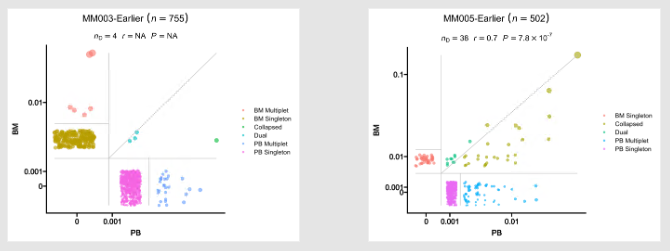
The points in the plot are jittered to avoid overplotting. The x-axis is the residency in the first group and
the y-axis is the residency in the second group. The size of the points are relative to the normalized size of
the clones. You may identify different types of clones in the plot based on their residency in the two groups:
- Collapsed (The clones that are collapsed in the second group)
- Dual (The clones that are present in both groups with equal size)
- Expanded (The clones that are expanded in the second group)
- First Group Multiplet (The clones only in the First Group with size > 1)
- Second Group Multiplet (The clones only in the Second Group with size > 1)
- First Group Singlet (The clones only in the First Group with size = 1)
- Second Group Singlet (The clones only in the Second Group with size = 1)
This idea is borrowed from this paper:
> [Wu, Thomas D., et al. "Peripheral T cell expansion predicts tumour infiltration and clinical response." Nature 579.7798 (2020): 274-278.](https://www.nature.com/articles/s41586-020-2056-8)
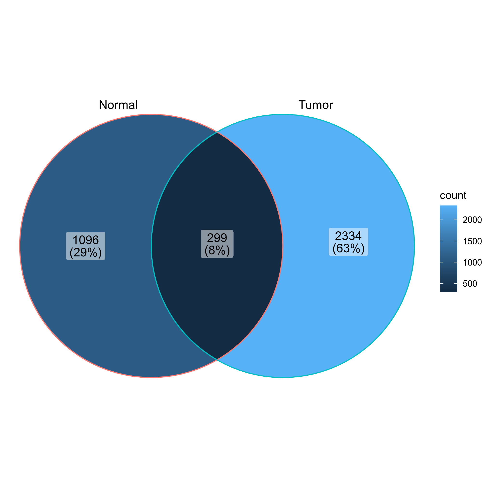
- Venn diagrams showing the overlap of the clones in the two groups
{: width="60%"}
Input:
immdata: The data loaded by `immunarch::repLoad()`
metafile: A cell-level metafile, where the first column must be the cell barcodes
that match the cell barcodes in `immdata`. The other columns can be any
metadata that you want to use for the analysis. The loaded metadata will be
left-joined to the converted cell-level data from `immdata`.
This can also be a Seurat object RDS file. If so, the `sobj@meta.data` will
be used as the metadata.
Output:
outdir: The output directory
Envs:
subject (list): The key of subject in metadata. The clone
residency will be examined for this subject/patient
group: The key of group in metadata. This usually marks the samples
that you want to compare. For example, Tumor vs Normal,
post-treatment vs baseline
It doesn't have to be 2 groups always. If there are more than 3
groups, instead of venn diagram, upset plots will be used.
order (list): The order of the values in `group`. In scatter/residency plots,
`X` in `X,Y` will be used as x-axis and `Y` will be used as y-axis.
You can also have multiple orders. For example: `["X,Y", "X,Z"]`.
If you only have two groups, you can set `order = ["X", "Y"]`, which will
be the same as `order = ["X,Y"]`.
section: How the subjects aligned in the report. Multiple subjects with
the same value will be grouped together.
Useful for cohort with large number of samples.
mutaters (type=json): The mutaters passed to `dplyr::mutate()` on
the cell-level data converted from `in.immdata`. If `in.metafile` is
provided, the mutaters will be applied to the joined data.
The keys will be the names of the new columns, and the values will be the
expressions. The new names can be used in `subject`, `group`, `order` and
`section`.
subset: The filter passed to `dplyr::filter()` to filter the data for the cells
before calculating the clone residency. For example, `Clones > 1` to filter
out singletons.
prefix: The prefix of the cell barcodes in the `Seurat` object.
upset_ymax: The maximum value of the y-axis in the upset bar plots.
upset_trans: The transformation to apply to the y axis of upset bar plots.
For example, `log10` or `sqrt`. If not specified, the y axis will be
plotted as is. Note that the position of the bar plots will be dodged
instead of stacked when the transformation is applied.
See also <https://github.com/tidyverse/ggplot2/issues/3671>
cases (type=json): If you have multiple cases, you can use this argument
to specify them. The keys will be used as the names of the cases.
The values will be passed to the corresponding arguments.
If no cases are specified, the default case will be added, with
the name `DEFAULT` and the values of `envs.subject`, `envs.group`,
`envs.order` and `envs.section`. These values are also the
defaults for the other cases.
""" # noqa: E501
input = "immdata:file,metafile:file"
output = "outdir:dir:{{in.immdata | stem}}.cloneov"
lang = config.lang.rscript
envs = {
"subject": [],
"group": None,
"order": [],
"section": None,
"mutaters": {},
"subset": None,
"prefix": "{Sample}_",
"upset_ymax": None,
"upset_trans": None,
"cases": {},
}
script = "file://../scripts/tcr/CloneResidency.R"
order = 2
plugin_opts = {"report": "file://../reports/tcr/CloneResidency.svelte"}
@mark(deprecated=True)DOCS
class Immunarch2VDJtools(Proc):
"""Convert immuarch format into VDJtools input formats.
This process converts the [`immunarch`](https://immunarch.com/) object to the
[`VDJtools`](https://vdjtools-doc.readthedocs.io/en/master/) input files,
in order to perform the VJ gene usage analysis by
[`VJUsage`](!!#biopipennstcrvjusage) process.
This process will generally generate a tab-delimited file for each sample,
with the following columns.
- `count`: The number of reads for this clonotype
- `frequency`: The frequency of this clonotype
- `CDR3nt`: The nucleotide sequence of the CDR3 region
- `CDR3aa`: The amino acid sequence of the CDR3 region
- `V`: The V gene
- `D`: The D gene
- `J`: The J gene
See also: <https://vdjtools-doc.readthedocs.io/en/master/input.html#vdjtools-format>.
This process has no environment variables.
Input:
immdata: The data loaded by `immunarch::repLoad()`
Output:
outdir: The output directory containing the vdjtools input for each
sample
""" # noqa: E501
input = "immdata:file"
output = "outdir:dir:{{in.immdata | stem}}.vdjtools_input"
lang = config.lang.rscript
script = "file://../scripts/tcr/Immunarch2VDJtools.R"
@mark(deprecated=True)DOCS
class ImmunarchSplitIdents(Proc):
"""Split the data into multiple immunarch datasets by Idents from Seurat
Note that only the cells in both the `immdata` and `sobjfile` will be
kept.
Requires `immunarch >= 0.9.0` to use `select_clusters()`
Input:
immdata: The data loaded by `immunarch::repLoad()`
sobjfile: The Seurat object file.
You can set a different ident by `Idents(sobj) <- "new_ident"` to
split the data by the new ident, where `"new_ident"` is the an
existing column in meta data
Output:
outdir: The output directory containing the RDS files of the splitted
immunarch datasets
Envs:
prefix: The prefix of the cell barcodes in the `Seurat` object.
Once could use a fixed prefix, or a placeholder with the column
name in meta data. For example, `"{Sample}_"` will replace the
placeholder with the value of the column `Sample` in meta data.
sample_col: The column name in meta data that contains the sample name
"""
input = "immdata:file, sobjfile:file"
output = "outdir:dir:{{in.immdata | stem}}.splitidents"
lang = config.lang.rscript
envs = {"prefix": "{Sample}_", "sample_col": "Sample"}
script = "file://../scripts/tcr/ImmunarchSplitIdents.R"
@mark(deprecated="{proc.name} is deprecated, use ClonalStats instead.")DOCS
class VJUsage(Proc):
"""Circos-style V-J usage plot displaying the frequency of
various V-J junctions using vdjtools.
This process performs the VJ gene usage analysis using
[`VDJtools`](https://vdjtools-doc.readthedocs.io/en/master/).
It wraps the [`PlotFancyVJUsage`](https://vdjtools-doc.readthedocs.io/en/master/basic.html#plotfancyvjusage) command in `VDJtools`.
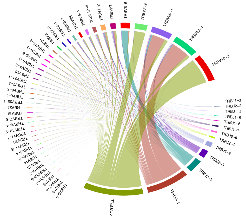
The output will be a V-J junction circos plot for a single sample.
Arcs correspond to different V and J segments, scaled to their frequency in sample.
Ribbons represent V-J pairings and their size is scaled to the pairing frequency
(weighted in present case).
{: width="80%" }
Input:
infile: The input file, in vdjtools input format
Output:
outfile: The V-J usage plot
Envs:
vdjtools: The path to the `VDJtools` executable.
vdjtools_patch (hidden): The patch file for `VDJtools`. It's delivered with the pipeline ([`biopipen`][3] package).
* You don't need to provide this file, unless you want to use a different patch file by yourself.
* See the issue with `VDJtools` [here](https://github.com/mikessh/vdjtools/issues/139).
""" # noqa: E501
input = "infile:file"
output = (
"outfile:file:{{ in.infile | stem | replace: '.vdjtools', '' }}"
".fancyvj.wt.png"
)
lang = config.lang.rscript
envs = {
"vdjtools": config.exe.vdjtools,
"vdjtools_patch": str(SCRIPT_DIR / "tcr" / "vdjtools-patch.sh"),
}
order = 3
script = "file://../scripts/tcr/VJUsage.R"
plugin_opts = {"report": "file://../reports/tcr/VJUsage.svelte"}
@mark(deprecated=True)DOCS
class Attach2Seurat(Proc):
"""Attach the clonal information to a Seurat object as metadata
Input:
immfile: The immunarch object in RDS
sobjfile: The Seurat object file in RDS
Output:
outfile: The Seurat object with the clonal information as metadata
Envs:
prefix: The prefix to the barcodes. You can use placeholder like
`{Sample}_` to use the meta data from the immunarch object
metacols: Which meta columns to attach
"""
input = "immfile:file, sobjfile:file"
output = "outfile:file:{{in.sobjfile | basename}}"
lang = config.lang.rscript
envs = {
"prefix": "{Sample}_",
"metacols": ["Clones", "Proportion", "CDR3.aa"],
}
script = "file://../scripts/tcr/Attach2Seurat.R"
class CDR3Clustering(Proc):DOCS
"""Cluster the TCR/BCR clones by their CDR3 sequences
This process is used to cluster TCR/BCR clones based on their CDR3 sequences.
It uses either
[GIANA](https://github.com/s175573/GIANA)
> Zhang, Hongyi, Xiaowei Zhan, and Bo Li.
> "GIANA allows computationally-efficient TCR clustering and multi-disease
> repertoire classification by isometric transformation."
> Nature communications 12.1 (2021): 1-11.
It is designed for TCR clustering, but it can also be used for BCR clustering.
See <https://github.com/s175573/GIANA/issues/18>.
Or [ClusTCR](https://github.com/svalkiers/clusTCR)
> Sebastiaan Valkiers, Max Van Houcke, Kris Laukens, Pieter Meysman,
> ClusTCR: a Python interface for rapid clustering of large sets of CDR3
> sequences with unknown antigen specificity,
> Bioinformatics, 2021.
Both methods are based on the
[Faiss Clustering Library](https://github.com/facebookresearch/faiss),
for efficient similarity search and clustering of dense vectors, so both methods
yield similar results.
A text file will be generated with the cluster assignments for each cell, together
with the `immunarch` object (in `R`) with the cluster assignments at `CDR3_Clsuter`
column. This information will then be merged to a `Seurat` object for further
downstream analysis.
The cluster assignments are prefixed with `S_` or `M_` to indicate whether a
cluster has only one unique CDR3 sequence or multiple CDR3 sequences.
Note that a cluster with `S_` prefix may still have multiple cells, as the same
CDR3 sequence may be shared by multiple cells.
Input:
screpfile: The TCR/BCR data object loaded by `scRepertoire::CombineTCR()`,
`scRepertoire::CombineBCR()` or `scRepertoire::CombineExpression()`
Output:
outfile: The `scRepertoire` object in qs with TCR/BCR cluster information.
Column `CDR3_Cluster` will be added to the metadata.
Envs:
type (choice): The type of the data.
- TCR: T cell receptor data
- BCR: B cell receptor data
- auto: Automatically detect the type from the data.
Try to find TRB or IGH genes in the CTgene column to determine
whether it is TCR or BCR data.
tool (choice): The tool used to do the clustering, either
[GIANA](https://github.com/s175573/GIANA) or
[ClusTCR](https://github.com/svalkiers/clusTCR).
For GIANA, using TRBV mutations is not supported
- GIANA: by Li lab at UT Southwestern Medical Center
- ClusTCR: by Sebastiaan Valkiers, etc
python: The path of python with `GIANA`'s dependencies installed
or with `clusTCR` installed. Depending on the `tool` you choose.
within_sample (flag): Whether to cluster the TCR/BCR clones within each sample.
When `in.screpfile` is a `Seurat` object, the samples are marked by
the `Sample` column in the metadata.
args (type=json): The arguments for the clustering tool
For GIANA, they will be passed to `python GIAna.py`
See <https://github.com/s175573/GIANA#usage>.
For ClusTCR, they will be passed to `clustcr.Clustering(...)`
See <https://svalkiers.github.io/clusTCR/docs/clustering/how-to-use.html#clustering>.
chain (choice): The TCR/BCR chain to use for clustering.
- heavy: The heavy chain, TRB for TCR, IGH for BCR.
For TCR, TRB is the second sequence in `CTaa`, separated by `_` if
input is a Seurat object; otherwise, it is extracted from the `cdr3_aa2` column.
For BCR, IGH is the first sequence in `CTaa`, separated by `_` if
input is a Seurat object; otherwise, it is extracted from the `cdr3_aa1` column.
- light: The light chain, TRA for TCR, IGL/IGK for BCR.
For TCR, TRA is the first sequence in `CTaa`, separated by `_` if
input is a Seurat object; otherwise, it is extracted from the `cdr3_aa1` column.
For BCR, IGL/IGK is the second sequence in `CTaa`, separated by `_` if
input is a Seurat object; otherwise, it is extracted from the `cdr3_aa2` column.
- TRA: Only the TRA chain for TCR (light chain).
- TRB: Only the TRB chain for TCR (heavy chain).
- IGH: Only the IGH chain for BCR (heavy chain).
- IGLK: Only the IGL/IGK chain for BCR (light chain).
- both: Both sequences from the heavy and light chains (CTaa column).
Requires:
clusTCR:
- if: {{ proc.envs.tool == 'ClusTCR' }}
- check: {{ proc.envs.python }} -c "import clustcr"
""" # noqa: E501
input = "screpfile:file"
output = "outfile:file:{{in.screpfile | stem}}.tcr_clustered.qs"
lang = config.lang.rscript
envs = {
"type": "auto", # or TCR, BCR
"tool": "GIANA", # or ClusTCR
"python": config.lang.python,
"within_sample": True, # whether to cluster the TCR clones within each sample
"args": {},
"chain": "both",
}
script = "file://../scripts/tcr/CDR3Clustering.R"
@mark(deprecated="{proc.name} is deprecated, use ClonalStats instead.")DOCS
class TCRClusterStats(Proc):
"""Statistics of TCR clusters, generated by `TCRClustering`.
The statistics include
- The number of cells in each cluster (cluster size)
- Sample diversity using TCR clusters instead of TCR clones
- Shared TCR clusters between samples
Examples:
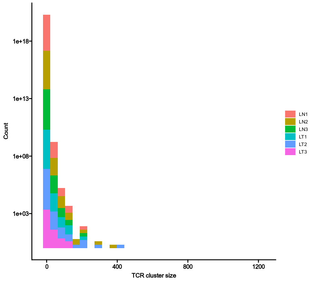
### Cluster size
```toml
[TCRClusterStats.envs.cluster_size]
by = "Sample"
```
{: width="80%"}
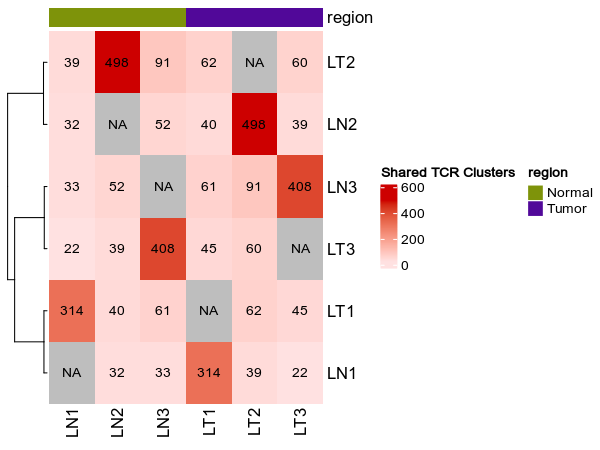
### Shared clusters
```toml
[TCRClusterStats.envs.shared_clusters]
numbers_on_heatmap = true
heatmap_meta = ["region"]
```
{: width="80%"}
### Sample diversity
```toml
[TCRClusterStats.envs.sample_diversity]
method = "gini"
```
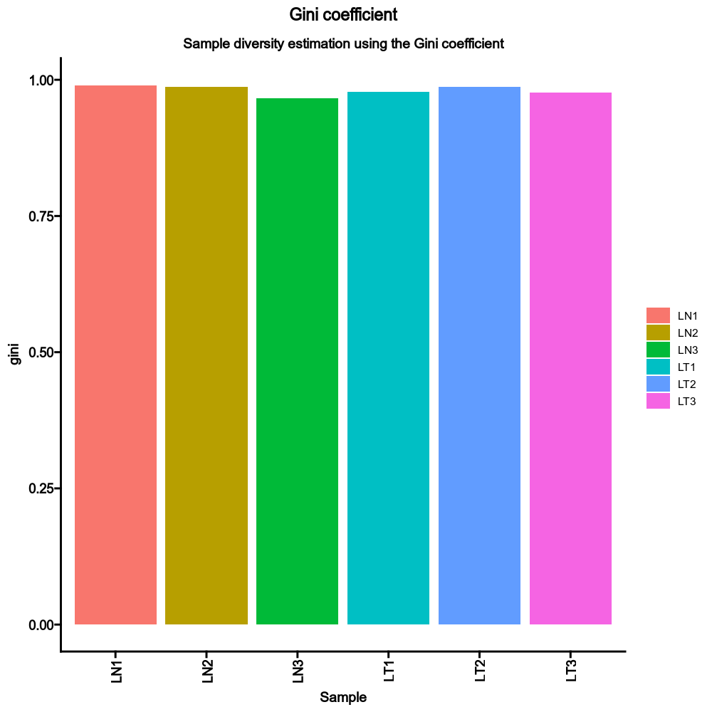{: width="80%"}
Compared to the sample diversity using TCR clones:
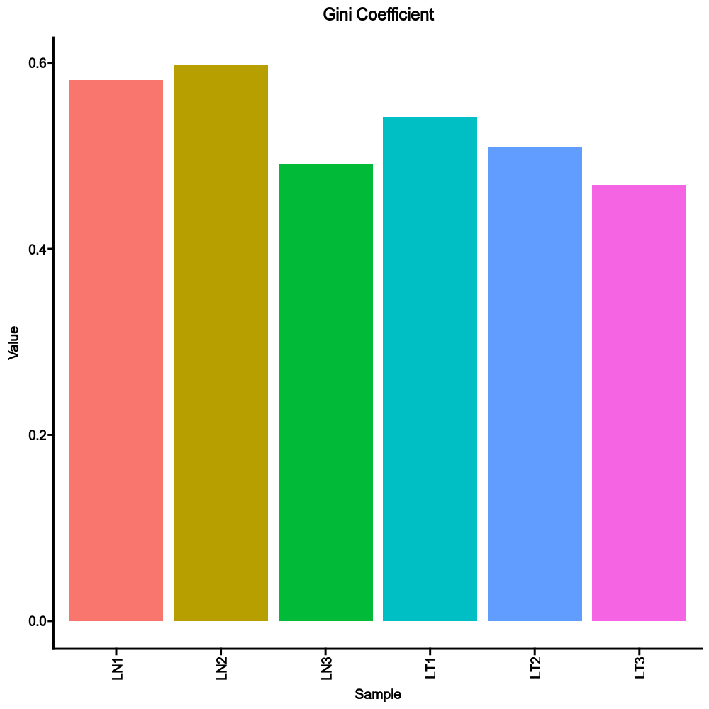{: width="80%"}
Input:
immfile: The immunarch object with TCR clusters attached
Output:
outdir: The output directory containing the stats and reports
Envs:
cluster_size (ns): The distribution of size of each cluster.
- by: The variables (column names) used to fill the histogram.
Only a single column is supported.
- devpars (ns): The parameters for the plotting device.
- width (type=int): The width of the device
- height (type=int): The height of the device
- res (type=int): The resolution of the device
- cases (type=json): If you have multiple cases, you can use this
argument to specify them. The keys will be the names of the
cases. The values will be passed to the corresponding arguments
above. If any of these arguments are not specified, the values
in `envs.cluster_size` will be used. If NO cases are
specified, the default case will be added, with the name
`DEFAULT`.
shared_clusters (ns): Stats about shared TCR clusters
- numbers_on_heatmap (flag): Whether to show the
numbers on the heatmap.
- heatmap_meta (list): The columns of metadata to show on the
heatmap.
- cluster_rows (flag): Whether to cluster the rows on the heatmap.
- sample_order: The order of the samples on the heatmap.
Either a string separated by `,` or a list of sample names.
This only works for columns if `cluster_rows` is `True`.
- grouping: The groups to investigate the shared clusters.
If specified, venn diagrams will be drawn instead of heatmaps.
In such case, `numbers_on_heatmap` and `heatmap_meta` will be
ignored.
- devpars (ns): The parameters for the plotting device.
- width (type=int): The width of the device
- height (type=int): The height of the device
- res (type=int): The resolution of the device
- cases (type=json): If you have multiple cases, you can use this
argument to specify them. The keys will be the names of the
cases. The values will be passed to the corresponding arguments
above. If any of these arguments are not specified, the values
in `envs.shared_clusters` will be used. If NO cases are
specified, the default case will be added, with the name
`DEFAULT`.
sample_diversity (ns): Sample diversity using TCR clusters instead of
clones.
- by: The variables (column names) to group samples.
Multiple columns should be separated by `,`.
- method (choice): The method to calculate diversity.
- gini: The Gini coefficient.
It measures the inequality among values of a frequency
distribution (for example levels of income).
- gini.simp: The Gini-Simpson index.
It is the probability of interspecific encounter, i.e.,
probability that two entities represent different types.
- inv.simp: Inverse Simpson index.
It is the effective number of types that is obtained when
the weighted arithmetic mean is used to quantify average
proportional abundance of types in the dataset of interest.
- div: true diversity, or the effective number of types.
It refers to the number of equally abundant types needed
for the average proportional abundance of the types to
equal that observed in the dataset of interest where all
types may not be equally abundant.
- devpars (ns): The parameters for the plotting device.
- width (type=int): The width of the device
- height (type=int): The height of the device
- res (type=int): The resolution of the device
- cases (type=json): If you have multiple cases, you can use this
argument to specify them. The keys will be the names of the
cases. The values will be passed to the corresponding arguments
above. If any of these arguments are not specified, the values
in `envs.sample_diversity` will be used. If NO cases are
specified, the default case will be added, with the name
`DEFAULT`.
Requires:
r-immunarch:
- check: {{proc.lang}} -e "library(immunarch)"
""" # noqa: E501
input = "immfile:file"
output = "outdir:dir:{{in.immfile | stem}}.tcrclusters_stats"
lang = config.lang.rscript
envs = {
"cluster_size": {
"by": "Sample",
"devpars": {"width": 1000, "height": 900, "res": 100},
"cases": {},
},
"shared_clusters": {
"numbers_on_heatmap": True,
"heatmap_meta": [],
"cluster_rows": True,
"sample_order": None,
"cluster_rows": True,
"grouping": None,
"devpars": {"width": 1000, "height": 1000, "res": 100},
"cases": {},
},
"sample_diversity": {
"by": None,
"method": "gini",
"devpars": {"width": 1000, "height": 1000, "res": 100},
"cases": {},
},
}
script = "file://../scripts/tcr/TCRClusterStats.R"
plugin_opts = {
"report": "file://../reports/tcr/TCRClusterStats.svelte",
}
@mark(deprecated=True)DOCS
class CloneSizeQQPlot(Proc):
"""QQ plot of the clone sizes
QQ plots for clones sizes of pairs of samples
Input:
immdata: The data loaded by `immunarch::repLoad()`
Output:
outdir: The output directory
Envs:
subject: The key of subject in metadata, defining the pairs.
The clone residency will be examined for this subject/patient
group: The key of group in metadata. This usually marks the samples
that you want to compare. For example, Tumor vs Normal,
post-treatment vs baseline
It doesn't have to be 2 groups always. If there are more than 3
groups, for example, [A, B, C], the QQ plots will be generated
for all the combinations of 2 groups, i.e., [A, B], [A, C], [B, C]
order: The order of the values in `group`. Early-ordered group will
be used as x-axis in scatter plots
If there are more than 2 groups, for example, [A, B, C], the
QQ plots will be drawn for pairs: B ~ A, C ~ B.
diag: Whether to draw the diagonal line in the QQ plot
on: The key of the metadata to use for the QQ plot. One/Both of
`["Clones", "Proportion"]`
"""
input = "immdata:file"
output = "outdir:dir:{{in.immdata | stem}}.qqplots"
lang = config.lang.rscript
envs = {
"subject": [],
"group": None,
"order": [],
"diag": True,
"on": ["Clones", "Proportion"],
}
script = "file://../scripts/tcr/CloneSizeQQPlot.R"
order = 3
plugin_opts = {"report": "file://../reports/tcr/CloneSizeQQPlot.svelte"}
class CDR3AAPhyschem(Proc):DOCS
"""CDR3 AA physicochemical feature analysis
The idea is to perform a regression between two groups of cells
(e.g. Treg vs Tconv) at different length of CDR3 AA sequences.
The regression will be performed for each physicochemical feature of the
AA (hydrophobicity, volume and isolectric point).
Reference:
- [Stadinski, Brian D., et al. "Hydrophobic CDR3 residues promote the development of self-reactive T cells." Nature immunology 17.8 (2016): 946-955.](https://www.nature.com/articles/ni.3491)
- [Lagattuta, Kaitlyn A., et al. "Repertoire analyses reveal T cell antigen receptor sequence features that influence T cell fate." Nature immunology 23.3 (2022): 446-457.](https://www.nature.com/articles/s41590-022-01129-x)
- [Wimley, W. C. & White, S. H. Experimentally determined hydrophobicity scale for proteins at membrane - interfaces. Nat. Struct. Biol. 3, 842-848 (1996).](https://www.nature.com/articles/nsb1096-842)
- [Handbook of chemistry & physics 72nd edition. (CRC Press, 1991).](https://books.google.com/books?hl=en&lr=&id=bNDMBQAAQBAJ&oi=fnd&pg=PP1&dq=Hdbk+of+chemistry+%26+physics&ots=H9fzwhwz-C&sig=EXHI9N3q4OW9TYEBWlldqkvADfM#v=onepage&q=Hdbk%20of%20chemistry%20%26%20physics&f=false)
- [Zamyatnin, A. A. Protein volume in solution. Prog. Biophys. Mol. Biol. 24, 107-123 (1972).](https://www.sciencedirect.com/science/article/pii/0079610772900053)
Input:
scrfile: The data loaded by `ScRepCombiningExpression`, saved in RDS or qs/qs2 format.
The data is actually generated by `scRepertiore::combineExpression()`.
The data must have both TRA and TRB chains.
Output:
outdir: The output directory
Envs:
group: The key of group in metadata to define the groups to
compare. For example, `CellType`, which has cell types annotated
for each cell in the combined object (immdata + Seurat metadata)
comparison (type=auto): A dict of two groups, with keys as the
group names and values as the group labels. For example,
```toml
Treg = ["CD4 CTL", "CD4 Naive", "CD4 TCM", "CD4 TEM"]
Tconv = "Tconv"
```
Or simply a list of two groups, for example, `["Treg", "Tconv"]` when
they are both in the `group` column.
target: Which group to use as the target group. The target
group will be labeled as 1, and the other group will be labeled as
0 in the regression.
If not specified, the first group in `comparison` will be used as
the target group.
each (auto): A column, or a list of columns or a string of columns separated by comma.
The columns will be used to split the data into multiple groups and the regression will be
applied to each group separately.
If not provided, all the cells will be used.
""" # noqa: E501
input = "scrfile:file"
output = "outdir:dir:{{in.immdata | stem}}.cdr3aaphyschem"
lang = config.lang.rscript
envs = {
"group": None,
"comparison": None,
"target": None,
"each": None,
}
script = "file://../scripts/tcr/CDR3AAPhyschem.R"
plugin_opts = {"report": "file://../reports/tcr/CDR3AAPhyschem.svelte"}
class TESSA(Proc):DOCS
"""Tessa is a Bayesian model to integrate T cell receptor (TCR) sequence
profiling with transcriptomes of T cells.
Enabled by the recently developed single cell sequencing techniques, which provide
both TCR sequences and RNA sequences of each T cell concurrently, Tessa maps the
functional landscape of the TCR repertoire, and generates insights into
understanding human immune response to diseases. As the first part of tessa,
BriseisEncoder is employed prior to the Bayesian algorithm to capture the TCR
sequence features and create numerical embeddings. We showed that the reconstructed
Atchley Factor matrices and CDR3 sequences, generated through the numerical
embeddings, are highly similar to their original counterparts. The CDR3 peptide
sequences are constructed via a RandomForest model applied on the reconstructed
Atchley Factor matrices.
See <https://github.com/jcao89757/TESSA>
When finished, two columns will be added to the `meta.data` of the `Seurat` object:
- `TESSA_Cluster`: The cluster assignments from TESSA.
- `TESSA_Cluster_Size`: The number of cells in each cluster.
These columns can be then used for further downstream analysis to explore the
functional landscape of the TCR repertoire.
Reference:
- 'Mapping the Functional Landscape of TCR Repertoire.',
Zhang, Z., Xiong, D., Wang, X. et al. 2021.
[link](https://www.nature.com/articles/s41592-020-01020-3)
- 'Deep learning-based prediction of the T cell receptor-antigen
binding specificity.', Lu, T., Zhang, Z., Zhu, J. et al. 2021.
[link](https://www.nature.com/articles/s42256-021-00383-2)
Input:
screpdata: The data loaded by `ScRepCombiningExpression`, saved in RDS or
qs/qs2 format.
The data is actually generated by `scRepertiore::combineExpression()`.
The data must have both TRA and TRB chains.
Output:
outfile: a qs fileof a Seurat object, with
`TESSA_Cluster` and `TESSA_Cluster_Size` added to the `meta.data`
Envs:
python: The path of python with `TESSA`'s dependencies installed
within_sample (flag): Whether the TCR networks are constructed only
within TCRs from the same sample/patient (True) or with all the
TCRs in the meta data matrix (False).
assay: Which assay to use to extract the expression matrix.
Only works if `in.srtobj` is an RDS file of a Seurat object.
By default, if `SCTransform` is performed, `SCT` will be used.
predefined_b (flag): Whether use the predefined `b` or not.
Please check the paper of tessa for more details about the b vector.
If True, the tessa will not update b in the MCMC iterations.
max_iter (type=int): The maximum number of iterations for MCMC.
save_tessa (flag): Save tessa detailed results to seurat object?
It will be saved to `sobj@misc$tessa`.
"""
input = "screpdata:file"
output = "outfile:file:{{in.screpdata | stem}}.tessa.qs"
lang = config.lang.rscript
envs = {
"python": config.lang.python,
"assay": None,
"within_sample": False,
"predefined_b": False,
"max_iter": 1000,
"save_tessa": False,
}
script = "file://../scripts/tcr/TESSA.R"
plugin_opts = {"report": "file://../reports/tcr/TESSA.svelte"}
class TCRDock(Proc):DOCS
"""Using TCRDock to predict the structure of MHC-peptide-TCR complexes
See <https://github.com/phbradley/TCRdock>.
Input:
configfile: The config file for TCRDock
It's should be a toml file with the keys listed in `envs`, including
`organism`, `mhc_class`, `mhc`, `peptide`, `va`, `ja`, `vb`, `jb`,
`cdr3a`, and `cdr3b`.
The values will overwrite the values in `envs`.
Output:
outdir: The output directory containing the results
Envs:
organism: The organism of the TCR, peptide and MHC
mhc_class (type=int): The MHC class, either `1` or `2`
mhc: The MHC allele, e.g., `A*02:01`
peptide: The peptide sequence
va: The V alpha gene
ja: The J alpha gene
vb: The V beta gene
jb: The J beta gene
cdr3a: The CDR3 alpha sequence
cdr3b: The CDR3 beta sequence
python: The path of python with dependencies for `tcrdock` installed.
If not provided, `TCRDock.lang` will be used (the same interpreter
used for the wrapper script).
It could also be a list to specify, for example, a python in a conda
environment (e.g., `["conda", "run", "-n", "myenv", "python"]`).
tmpdir: The temporary directory used to clone the `tcrdock` source code if
`envs.tcrdock` is not provided.
tcrdock: The path to the `tcrdock` source code repo.
You need to clone the source code from the github repository.
<https://github.com/phbradley/TCRdock> at
revision c5a7af42eeb0c2a4492a4d4fe803f1f9aafb6193 at main branch.
You also have to run `download_blast.py` after cloning to download the
blast database in the directory.
If not provided, we will clone the source code to the `envs.tmpdir`
directory and run the `download_blast.py` script.
model_name: The model name to use
model_file: The model file to use.
If provided as a relative path, it should be relative to the
`<envs.data_dir>/params/`, otherwise, it should be the full path.
data_dir: The data directory that contains the model files.
The model files should be in the `params` subdirectory.
"""
input = "configfile:file"
output = "outdir:dir:{{in.configfile | stem}}.tcrdock"
lang = config.lang.python
envs = {
"tcrdock": None,
"organism": "human",
"mhc_class": 1,
"mhc": "A*02:01",
"peptide": None,
"va": None,
"ja": None,
"vb": None,
"jb": None,
"cdr3a": None,
"cdr3b": None,
"python": None,
"model_name": "model_2_ptm_ft4",
"model_file": "tcrpmhc_run4_af_mhc_params_891.pkl",
"data_dir": None,
}
script = "file://../scripts/tcr/TCRDock.py"
class ScRepLoading(Proc):DOCS
"""Load the single cell TCR/BCR data into a `scRepertoire` compatible object
This process loads the single cell TCR/BCR data into a `scRepertoire`
(>= v2.0.8, < v2.3.2) compatible object. Later, `scRepertoire::combineExpression`
can be used to combine the expression data with the TCR/BCR data.
For the data path specified at `TCRData`/`BCRData` in the input file
(`in.metafile`), will be used to find the TCR/BCR data files and
`scRepertoire::loadContigs()` will be used to load the data.
A directory can be specified in `TCRData`/`BCRData`, then
`scRepertoire::loadContigs()` will be used directly to load the data from the
directory. Otherwise if a file is specified, it will be symbolically linked to
a directory for `scRepertoire::loadContigs()` to load.
Note that when the file name can not be recognized by `scRepertoire::loadContigs()`,
`envs.format` must be set for the correct format of the data.
Input:
metafile: The meta data of the samples
A tab-delimited file
Two columns are required:
* `Sample` to specify the sample names.
* `TCRData`/`BCRData` to assign the path of the data to the samples,
and this column will be excluded as metadata.
Output:
outfile: The `scRepertoire` compatible object in qs/qs2 format
Envs:
type (choice): The type of the data to load.
- TCR: T cell receptor data
- BCR: B cell receptor data
- auto: Automatically detect the type from the metadata.
If `auto` is selected, the type will be determined by the presence of
`TCRData` or `BCRData` columns in the metadata. If both columns are
present, `TCR` will be selected by default.
combineTCR (type=json): The extra arguments for `scRepertoire::combineTCR`
function.
See also <https://www.borch.dev/uploads/screpertoire/reference/combinetcr>
combineBCR (type=json): The extra arguments for `scRepertoire::combineBCR`
function.
See also <https://www.borch.dev/uploads/screpertoire/reference/combinebcr>
exclude (auto): The columns to exclude from the metadata to add to the object.
A list of column names to exclude or a string with column names separated
by `,`. By default, `BCRData`, `TCRData` and `RNAData` will be excluded.
tmpdir: The temporary directory to store the symbolic links to the
TCR/BCR data files.
format (choice): The format of the TCR/BCR data files.
- 10X: 10X Genomics data, which is usually in a directory with
`filtered_contig_annotations.csv` file.
- AIRR: AIRR format, which is usually in a file with
`airr_rearrangement.tsv` file.
- BD: Becton Dickinson data, which is usually in a file with
`Contigs_AIRR.tsv` file.
- Dandelion: Dandelion data, which is usually in a file with
`all_contig_dandelion.tsv` file.
- Immcantation: Immcantation data, which is usually in a file with
`data.tsv` file.
- JSON: JSON format, which is usually in a file with `.json` extension.
- ParseBio: ParseBio data, which is usually in a file with
`barcode_report.tsv` file.
- MiXCR: MiXCR data, which is usually in a file with `clones.tsv` file.
- Omniscope: Omniscope data, which is usually in a file with `.csv`
extension.
- TRUST4: TRUST4 data, which is usually in a file with
`barcode_report.tsv` file.
- WAT3R: WAT3R data, which is usually in a file with
`barcode_results.csv` file.
See also: <https://rdrr.io/github/ncborcherding/scRepertoire/man/loadContigs.html>
If not provided, the format will be guessed from the file name by `scRepertoire::loadContigs()`.
""" # noqa: E501
input = "metafile:file"
output = "outfile:file:{{in.metafile | stem}}.scRep.qs"
lang = config.lang.rscript
envs = {
"type": "auto", # or TCR/BCR
"combineTCR": {"samples": True},
"combineBCR": {"samples": True},
"exclude": ["BCRData", "TCRData", "RNAData"],
"format": None,
"tmpdir": config.path.tmpdir,
}
script = "file://../scripts/tcr/ScRepLoading.R"
class ScRepCombiningExpression(Proc):DOCS
"""Combine the scTCR/BCR data with the expression data
This process combines the scTCR/BCR data with the expression data using
`scRepertoire::combineExpression` function. The expression data should be
in `Seurat` format. The `scRepertoire` object should be a combined contig
object, usually generated by `scRepertoire::combineTCR` or
`scRepertoire::combineBCR`.
See also: <https://www.borch.dev/uploads/screpertoire/reference/combineexpression>.
Input:
screpfile: The `scRepertoire` object in RDS/qs format
srtobj: The `Seurat` object, saved in RDS/qs format
Output:
outfile: The `Seurat` object with the TCR/BCR data combined
In addition to the meta columns added by
`scRepertoire::combineExpression()`, a new column `VDJ_Presence` will be
added to the metadata. It indicates whether the cell has a TCR/BCR
sequence or not. The value is `TRUE` if the cell has a TCR/BCR sequence,
and `FALSE` otherwise.
Envs:
cloneCall: How to call the clone - VDJC gene (gene), CDR3 nucleotide (nt),
CDR3 amino acid (aa), VDJC gene + CDR3 nucleotide (strict) or
a custom variable in the data.
chain: indicate if both or a specific chain should be used
e.g. "both", "TRA", "TRG", "IGH", "IGL".
group_by: The column label in the combined clones in which clone frequency will
be calculated. NULL or "none" will keep the format of input.data.
proportion (flag): Whether to proportion (TRUE) or total frequency (FALSE) of
the clone based on the group_by variable.
filterNA (flag): Method to subset Seurat/SCE object of barcodes without clone
information
cloneSize (type=json): The bins for the grouping based on proportion or
frequency.
If proportion is FALSE and the cloneSizes are not set high enough based on
frequency, the upper limit of cloneSizes will be automatically updated.
addLabel (flag): This will add a label to the frequency header, allowing the
user to try multiple group_by variables or recalculate frequencies after
subsetting the data.
"""
input = "screpfile:file,srtobj:file"
output = "outfile:file:{{in.screpfile | stem}}.qs"
lang = config.lang.rscript
envs = {
"cloneCall": "aa",
"chain": "both",
"group_by": "Sample",
"proportion": True,
"filterNA": False,
"cloneSize": {
"Rare": 1e-04,
"Small": 0.001,
"Medium": 0.01,
"Large": 0.1,
"Hyperexpanded": 1,
},
"addLabel": False,
}
script = "file://../scripts/tcr/ScRepCombiningExpression.R"
class ClonalStats(Proc):DOCS
"""Visualize the clonal information.
Using [`scplotter`](https://github.com/pwwang/scplotter) to visualize the clonal
information.
Examples:
### Clonal Volume
```toml
[ClonalStats.envs.cases."Clonal Volume"]
viz_type = "volume"
x_text_angle = 45
```
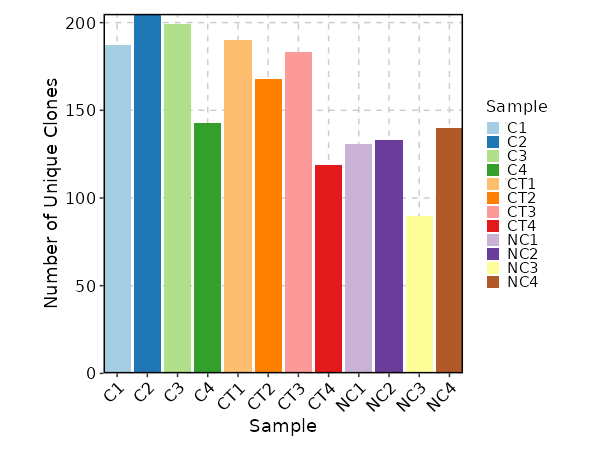{: width="80%"}
### Clonal Volume by Diagnosis
```toml
[ClonalStats.envs.cases."Clonal Volume by Diagnosis"]
viz_type = "volume"
x = "seurat_clusters"
group_by = "Diagnosis"
comparisons = true
```
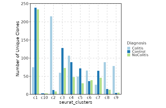{: width="80%"}
### Clonal Abundance
```toml
[ClonalStats.envs.cases."Clonal Abundance"]
viz_type = "abundance"
```
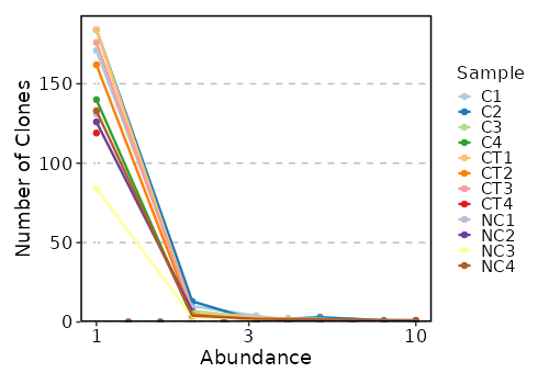{: width="80%"}
### Clonal Abundance Density
```toml
[ClonalStats.envs.cases."Clonal Abundance Density"]
viz_type = "abundance"
plot_type = "density"
```
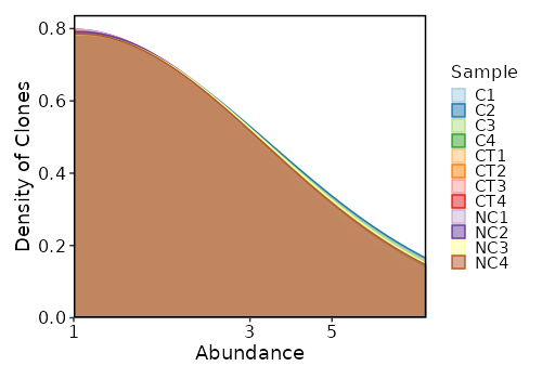{: width="80%"}
### CDR3 Length
```toml
[ClonalStats.envs.cases."CDR3 Length"]
viz_type = "length"
```
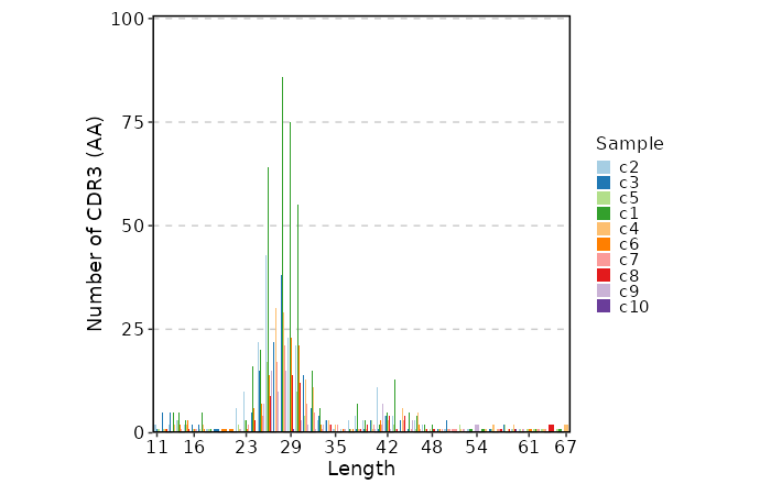{: width="80%"}
### CDR3 Length (Beta Chain)
```toml
[ClonalStats.envs.cases."CDR3 Length (Beta Chain)"]
viz_type = "length"
chain = "TRB"
```
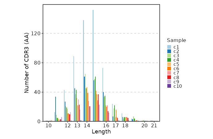{: width="80%"}
### Clonal Residency
```toml
[ClonalStats.envs.cases."Clonal Residency"]
viz_type = "residency"
group_by = "Diagnosis"
chain = "TRB"
clone_call = "gene"
groups = ["Colitis", "NoColitis"]
```
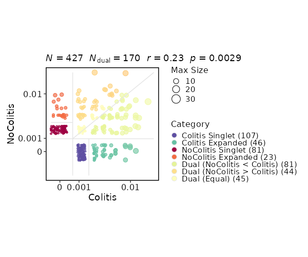{: width="80%"}
### Clonal Residency (UpSet Plot)
```toml
[ClonalStats.envs.cases."Clonal Residency (UpSet Plot)"]
viz_type = "residency"
plot_type = "upset"
group_by = "Diagnosis"
chain = "TRB"
clone_call = "gene"
groups = ["Colitis", "NoColitis"]
devpars = {width = 800}
```
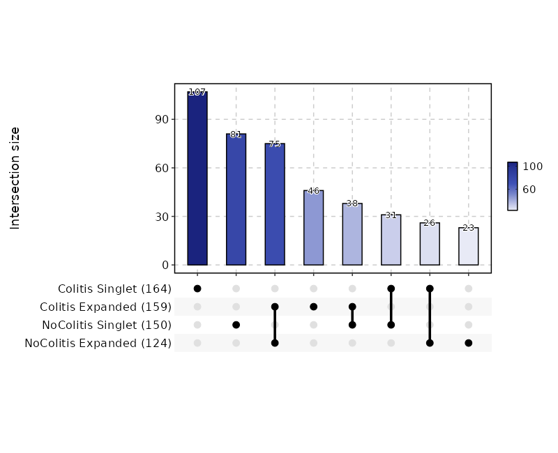{: width="80%"}
### Clonal Statistics with Expanded Clones
```toml
[ClonalStats.envs.cases."Clonal Statistics with Expanded Clones"]
viz_type = "stat"
plot_type = "pies"
group_by = "Diagnosis"
groups = ["Colitis", "NoColitis"]
clones = {"Expanded Clones In Colitis" = "sel(Colitis > 2)", "Expanded Clones In NoColitis" = "sel(NoColitis > 2)"}
subgroup_by = "seurat_clusters"
pie_size = "sqrt"
show_row_names = true
show_column_names = true
devpars = {width = 720}
```
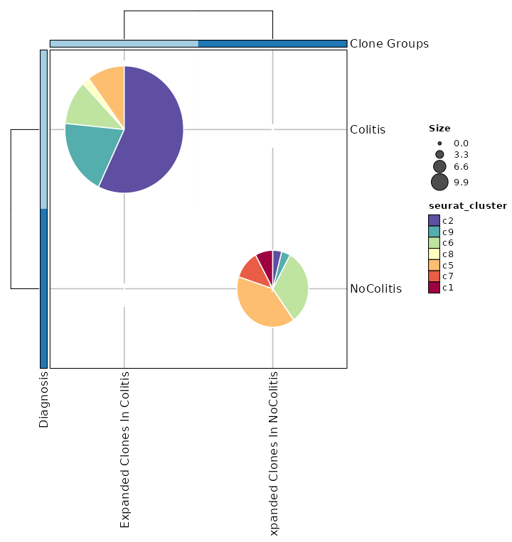{: width="80%"}
### Hyperexpanded Clonal Dynamics
```toml
[ClonalStats.envs.cases."Hyperexpanded Clonal Dynamics"]
viz_type = "stat"
plot_type = "sankey"
group_by = "Diagnosis"
chain = "TRB"
groups = ["Colitis", "NoColitis"]
clones = {"Hyper-Expanded Clones In Colitis" = "sel(Colitis > 5)", "Hyper-Expanded Clones In NoColitis" = "sel(NoColitis > 5)"}
devpars = {width = 800}
```
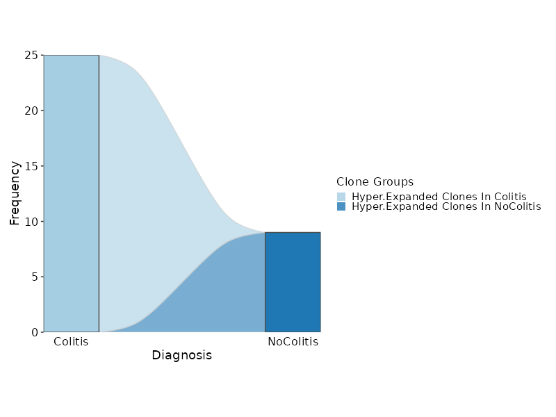{: width="80%"}
### Clonal Composition
```toml
[ClonalStats.envs.cases."Clonal Composition"]
viz_type = "composition"
x_text_angle = 45
```
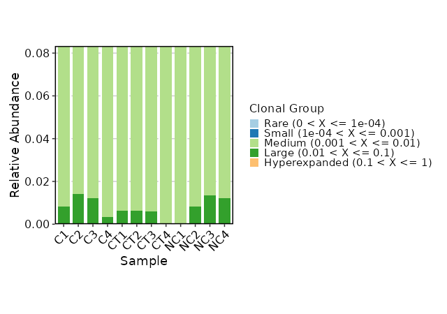{: width="80%"}
### Clonal Overlapping
```toml
viz_type = "overlap"
chain = "TRB"
clone_call = "gene"
```
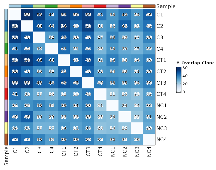{: width="80%"}
### Clonal Diversity
```toml
[ClonalStats.envs.cases."Clonal Diversity"]
# method = "shannon" # default
viz_type = "diversity"
x_text_angle = 45
```
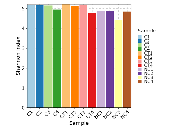{: width="80%"}
### Clonal Diversity (gini.coeff, by Diagnosis)
```toml
[ClonalStats.envs.cases."Clonal Diversity (gini.coeff, by Diagnosis)"]
method = "gini.coeff"
viz_type = "diversity"
plot_type = "box"
group_by = "Diagnosis"
comparisons = true
devpars = {height = 600, width = 600}
```
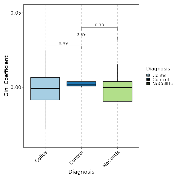{: width="80%"}
### Gene Usage Frequency
```toml
[ClonalStats.envs.cases."Gene Usage Frequency"]
viz_type = "geneusage"
devpars = {width = 1200}
```
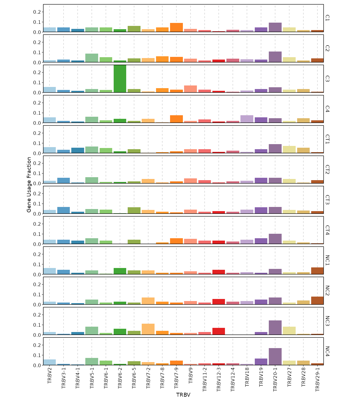{: width="80%"}
### Positional amino acid frequency
```toml
[ClonalStats.envs.cases."Positional amino acid frequency"]
viz_type = "positional"
# method = "AA" # default
devpars = {width = 1600}
```
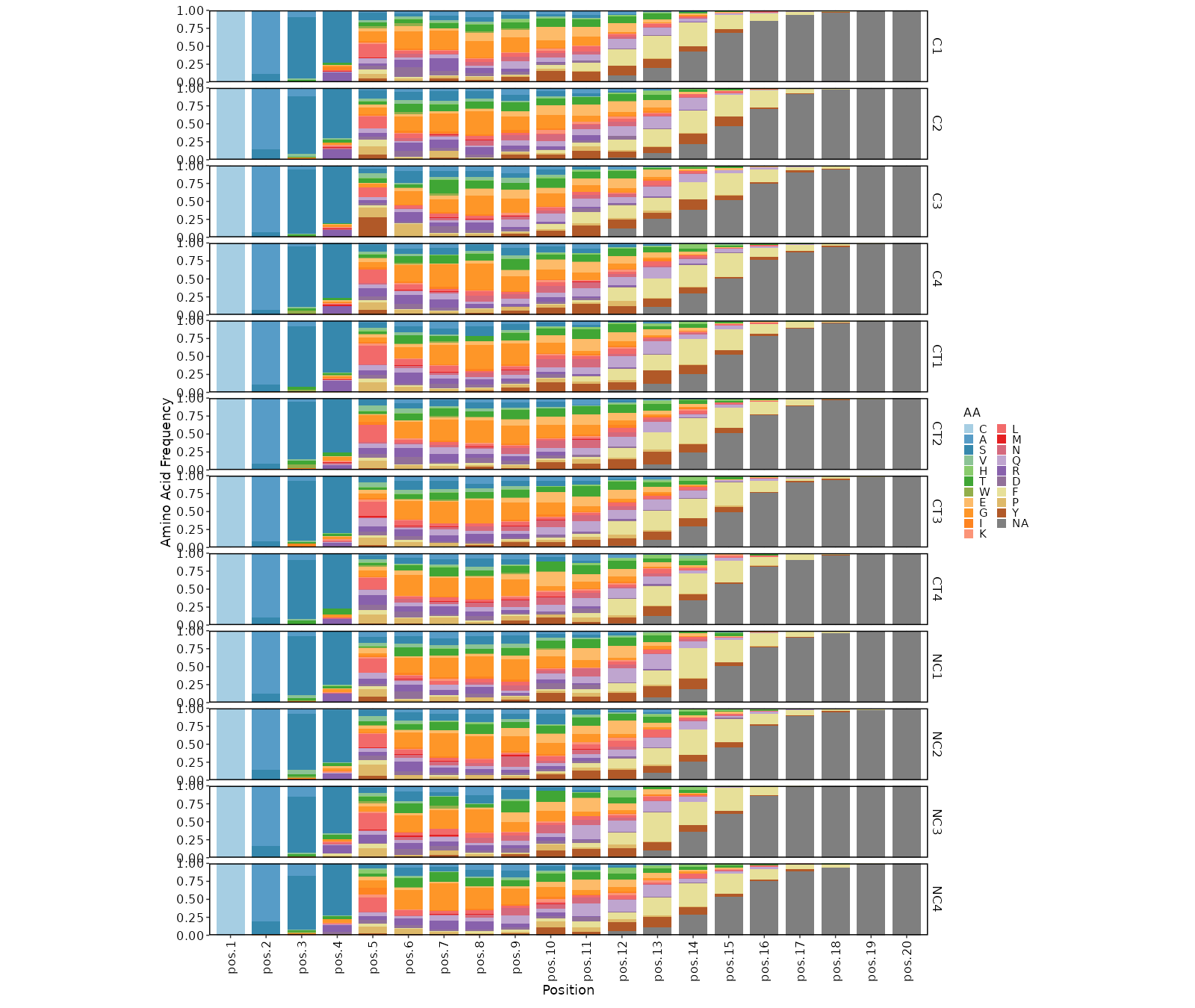{: width="80%"}
### Positional shannon entropy
```toml
[ClonalStats.envs.cases."Positional shannon entropy"]
viz_type = "positional"
method = "shannon"
devpars = {width = 1200}
```
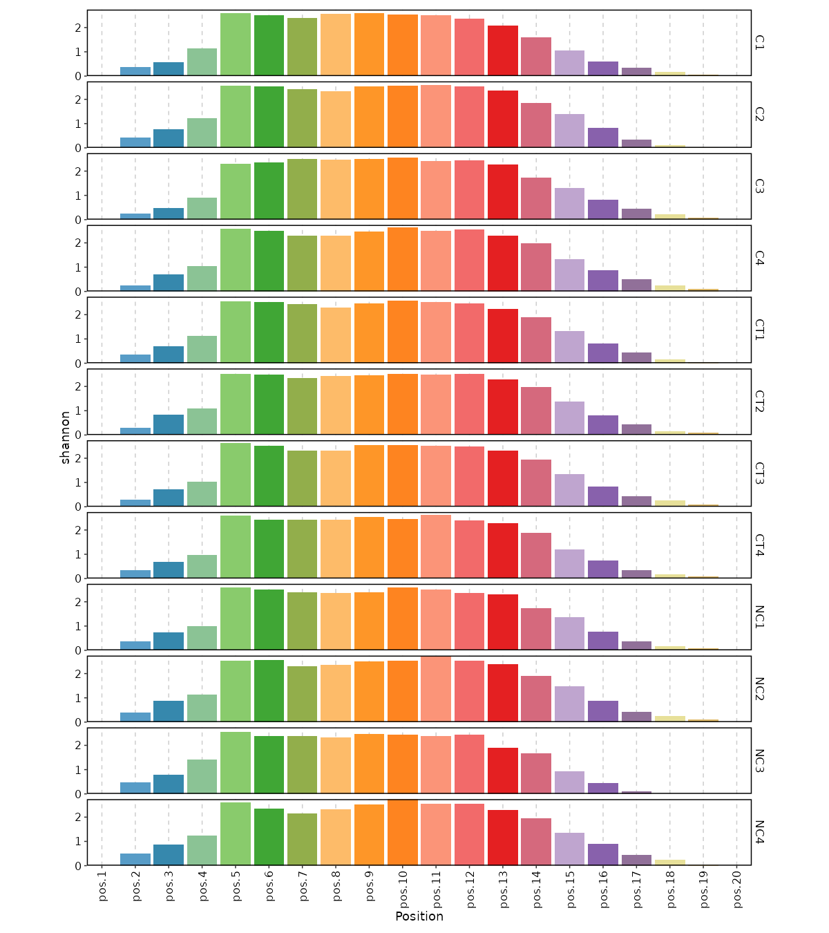{: width="80%"}
### 3-Mer Frequency
```toml
[ClonalStats.envs.cases."3-Mer Frequency"]
viz_type = "kmer"
k = 3 # default is 3
devpars = {width = 800}
```
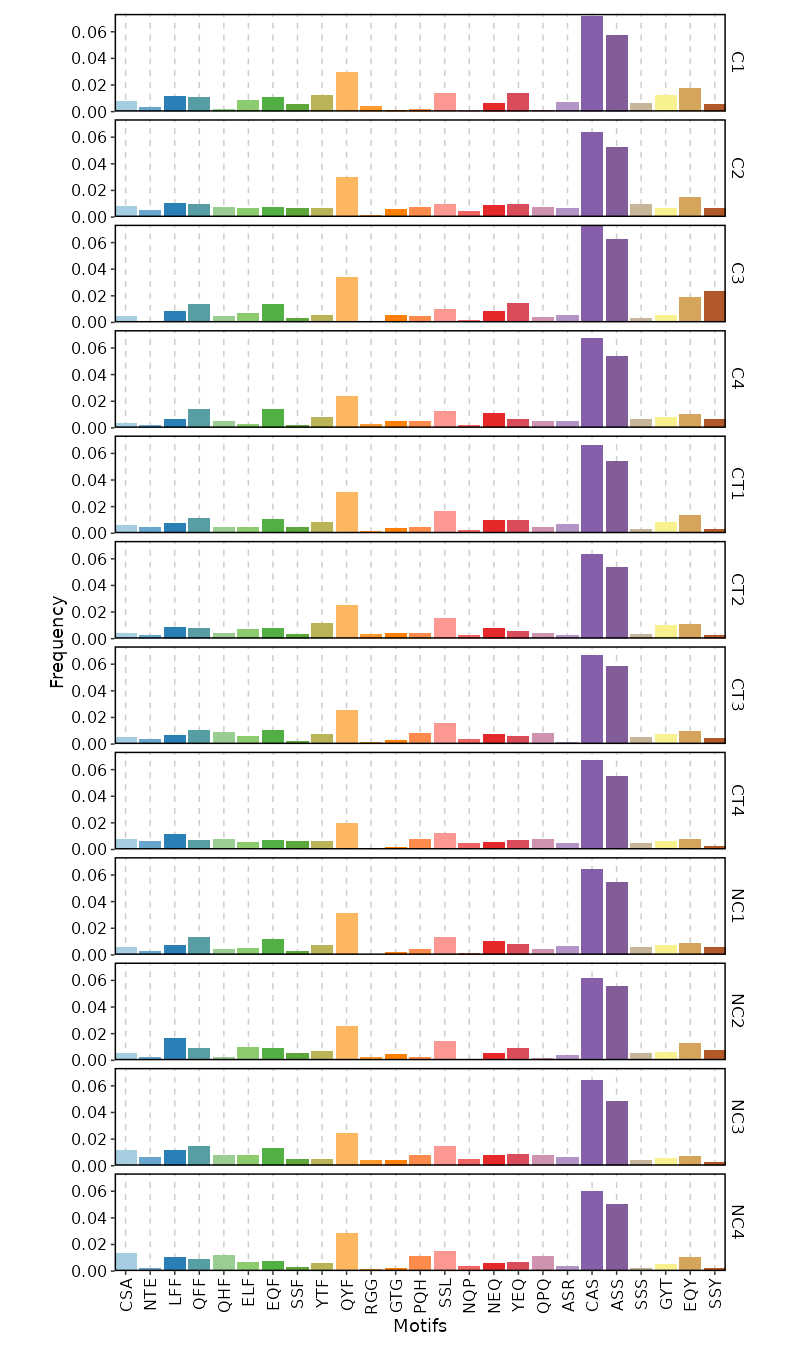{: width="80%"}
### Rarefaction Curve
```toml
[ClonalStats.envs.cases."Rarefaction Curve"]
viz_type = "rarefaction"
```
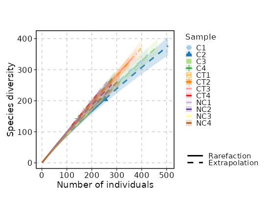{: width="80%"}
Input:
screpfile: The `scRepertoire` object in RDS/qs format
Output:
outdir: The output directory containing the plots
Envs:
mutaters (type=json;order=-9): The mutaters passed to `dplyr::mutate()` to add new variables.
When the object loaded form `in.screpfile` is a list, the mutaters will be applied to each element.
The keys are the names of the new variables, and the values are the expressions.
When it is a `Seurat` object, typically an output of `scRepertoire::combineExpression()`,
the mutaters will be applied to the `meta.data`.
cache (type=auto): Whether to cache the plots.
Currently only plots for features are supported, since creating the those
plots can be time consuming.
If `True`, the plots will be cached in the job output directory, which will
be not cleaned up when job is rerunning.
viz_type (choice): The type of visualization to generate.
- volume: The volume of the clones using [`ClonalVolumePlot`](https://pwwang.github.io/scplotter/reference/ClonalVolumePlot.html)
- abundance: The abundance of the clones using [`ClonalAbundancePlot`](https://pwwang.github.io/scplotter/reference/ClonalAbundancePlot.html)
- length: The length of the CDR3 sequences using [`ClonalLengthPlot`](https://pwwang.github.io/scplotter/reference/ClonalLengthPlot.html)
- residency: The residency of the clones using [`ClonalResidencyPlot`](https://pwwang.github.io/scplotter/reference/ClonalResidencyPlot.html)
- stat: The stats of the clones using [`ClonalStatPlot`](https://pwwang.github.io/scplotter/reference/ClonalStatPlot.html)
- composition: The composition of the clones using [`ClonalCompositionPlot`](https://pwwang.github.io/scplotter/reference/ClonalCompositionPlot.html)
- overlap: The overlap of the clones using [`ClonalOverlapPlot`](https://pwwang.github.io/scplotter/reference/ClonalOverlapPlot.html)
- diversity: The diversity of the clones using [`ClonalDiversityPlot`](https://pwwang.github.io/scplotter/reference/ClonalDiversityPlot.html)
- geneusage: The gene usage of the clones using [`ClonalGeneUsagePlot`](https://pwwang.github.io/scplotter/reference/ClonalGeneUsagePlot.html)
- positional: The positional information of the clones using [`ClonalPositionalPlot`](https://pwwang.github.io/scplotter/reference/ClonalPositionalPlot.html)
- kmer: The kmer information of the clones using [`ClonalKmerPlot`](https://pwwang.github.io/scplotter/reference/ClonalKmerPlot.html)
- rarefaction: The rarefaction curve of the clones using [`ClonalRarefactionPlot`](https://pwwang.github.io/scplotter/reference/ClonalRarefactionPlot.html)
subset: An expression to subset the data before plotting.
Similar to `mutaters`, it will be applied to each element by `dplyr::filter()` if the object
loaded form `in.screpfile` is a list; otherwise, it will be applied to
`subset(sobj, subset = <expr>)` if the object is a `Seurat` object.
devpars (ns): The parameters for the plotting device.
- width (type=int): The width of the device
- height (type=int): The height of the device
- res (type=int): The resolution of the device
more_formats (list): The extra formats to save the plots in, other than PNG.
save_code (flag): Whether to save the code used to generate the plots
Note that the data directly used to generate the plots will also be saved in an `rda` file.
Be careful if the data is large as it may take a lot of disk space.
save_data (flag): Whether to save the data used to generate the plot.
descr: The description of the plot, used to show in the report.
<more>: The arguments for the plot function
See the documentation of the corresponding plot function for the details
cases (type=json): The cases to generate the plots if we have multiple cases.
The keys are the names of the cases, and the values are the arguments for the plot function.
The arguments in `envs` will be used if not specified in `cases`, except for `mutaters`.
Sections can be specified as the prefix of the case name, separated by `::`.
For example, if you have a case named `Clonal Volume::Case1`, the plot will be put in the
section `Clonal Volume`. By default, when there are multiple cases for the same 'viz_type', the name of the 'viz_type' will be used
as the default section name (for example, when 'viz_type' is 'volume', the section name will be 'Clonal Volume').
When there is only a single case, the section name will default to 'DEFAULT', which will not be shown
in the report.
""" # noqa: E501
input = "screpfile:file"
output = "outdir:dir:{{in.screpfile | stem}}.clonalstats"
lang = config.lang.rscript
envs = {
"mutaters": {},
"cache": config.path.tmpdir,
"subset": None,
"viz_type": None,
"devpars": {"width": None, "height": None, "res": 100},
"more_formats": [],
"save_code": False,
"save_data": False,
"descr": None,
"cases": {
"Clonal Volume": {"viz_type": "volume"},
"Clonal Abundance": {"viz_type": "abundance"},
"CDR3 Length": {"viz_type": "length"},
"Clonal Diversity": {"viz_type": "diversity"},
}
}
script = "file://../scripts/tcr/ClonalStats.R"
plugin_opts = {"report": "file://../reports/tcr/ClonalStats.svelte"}